Day 42: Conditional Probability

How does this not exist on the internet?! This is directly from my book, so it looks a little… well loved.

Up to now we’ve been dealing with single variable pdf and the corresponding CDF. We said that these probabilities relied on the fact that our variable of interest was independent. However, what if we knew some property that impacted our probability? Today we are talking conditional probability and that is the question we will be answering. It’s going to be a long, long post so plan accordingly.*

Despite my best efforts, the internet seems to be lacking a good example of what a pdf that is conditional looks like. WTF internet, WTF. Well we’re going to fix that with an awful drawing of what having a conditioning statement attached to a pdf does to that pdf. It will make sense, don’t sweat it! Today will be a bit math heavy, but we can go step by step and hopefully we can make sense of it all!

First let’s review, you’ll probably want to read our posts on independence and specifically you’ll want to know about Bayes’ theorem, I told you we were bringing it back and I meant it. In fact, Bayes’ theorem is exactly why this works out the way it does, so having a good background will help.

Now that we’ve reviewed let’s look at what a conditioning statement is. When we have a dependent variable, we are literally saying that the value one variable has, changes the probability of another variable. We write this out like this

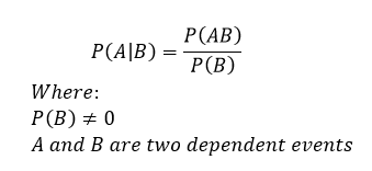
If you recall from our Bayes’ theorem we read P(A|B) as the probability of A given B. The only real constraint is that P(B) cannot be zero, this should be apparent why, but if P(B) was zero then we have the trivial solution, everything is zero.

Side note moving forward, when we start talking pdf we will be using the variable f and when we mean CDF we use F, this is standard in textbooks and you should be familiar with it, but we like being explicit around here, so moving forward keep this in mind so you don’t get confused because we will be going back and forth.

Most of these concepts work best with an example, so let’s take a look at the general example (meaning this is completely arbitrary so you can’t use it for anything real, but it shows you how the concept works). Say we wish to find the conditional distribution of a  random variable x assuming that x ≤ a is a number such that F(a) ≠ 0. This is just a math way of saying that our CDF of a cannot be zero (if it did we don’t have anything to show, so we are just being rigorous in our definition). So now (using our A and B for events) we have something like this:

B = {x ≤ a}

So now we want to find the pdf (f) and the CDF (F) and we can write that mathematically like this:

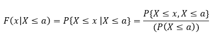
This is just saying that our CDF is a function F of x and we are selecting x to be some value X (capital X) less than or equal to a. Then we say that is equivalent to saying that we are interested in the probability P as X approaches x given that X is less than or equal to a, a fancy way of setting our x (which is the value in the equation) to the value we are interested in, which is X. Yes, the notation is confusing, but just remember that X (capital) is our input value for x (lowercase).

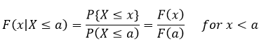
Next we say that is just equivalent to Bayes’ theorem where we plug in our values. Remember we have two conditions here, one where X ≤ x and one where X ≤ a, and we are saying that X ≤ x given that X is also less than or equal to a. Okay hopefully that clears that up. Using this relationship we already know something about the function, if x < a, then we can rewrite it like this { X ≤ x, x ≤ a} = { X ≤ x}. Which means

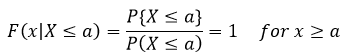
We can do this because we expressed F(x|B) in terms of the random variable x, so by having some knowledge of F(x) we can determine things about F(x|B) without having done anything with B (hence why it hasn’t shown up … yet). Basically what we are saying here is that the probability of event A happening given A happened is 100% or 1. This may seem redundant, but it actually does something important and tells us how our conditioning statement effects F(x). So now we know that our F(x|X≤a) looks something like this in relation to our F(x), remember this is representative so we don’t know exactly, but we have a good guess at this point what it looks like (at least at a).

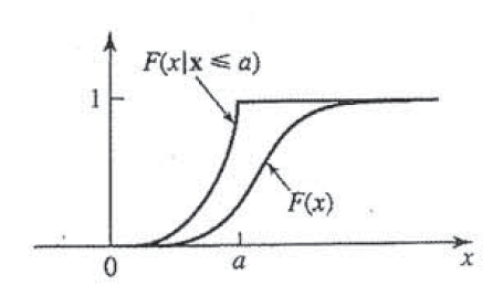
Notice that our F(x|X≤a) is larger than our F(x) this should make sense since we are saying that the probability that A will occur is higher if B has occurred.

We can do this going the other direction too and determine where our probability is zero and then we have a range for our function that is interesting (in that it isn’t zero or 100%). Let’s look at the other end of the equation though, what happens when x < a? In this case, if x < a then {X ≤ x, x ≤ a} = {X ≤ a}, which we plug into the original equation (just like we did for the last step) and we find

At first glance this doesn’t have anything fall out at us, but we can differentiate F(x|x≤ a) with respect to x and we can find the density (since we’ve already said that F'(x) = f(x), or to go from pdf to CDF we integrate, so going from CDF to pdf we take the derivative). So now we can find f(x) which gives us:

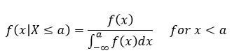
Now if you’re adept at math, you will see that this is 0 when x≥a. Don’t feel bad if you didn’t see that, neither did I at first. If you’re like me and want to understand why this is, it is basically because we are integrating from -∞ up to a value “a” so if x is larger than “a” there isn’t anything to integrate because everything is happening outside the range we are integrating (so the result is zero).

Well if you’ve made it this far and aren’t too badly confused, let’s see if we can get our conditional statement worked out. Up to this point we’ve related B to x and a by the relationship at the top, this guy:

B = {x ≤ a}

We’ve found the CDF or in this case F(x) for as far as we can go without plugging real numbers in and what not. However, this was with only one limitation to what x could be, what happens if we give it two? In this case let’s say that

B = {b < x ≤ a}

In this case we find that

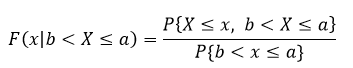
This is a very fancy way of saying that we are limiting our values that we can put into the equation to values between b and a (where X is the value we are putting into the equation. Now we can do the same few steps that we did above and derive what our extremes look like. Let’s look at when x ≥ a, in that case what follows is that {X ≤ x, b < X ≤ a} = {b < X ≤ a}. Which we then plug back into the equation such that

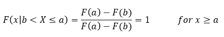
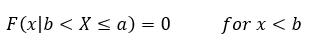
This is just saying once again the probability that something occurs after it occurred is 1, this helps us set the limit to the conditional statement because everything after this is just 1 and anything before this is some other value. This in particular came about because we said that X is bounded by a and b so if x is greater than or equal to a then it occurred and if it is less than b (our lower limit) then it has not occurred. In fact, let’s look at that case next, in this case if x < b, then {X ≤ x, b < X ≤ a} = {∅}. That ∅ just represent the null set, a fancy math way of saying that there is nothing in it. It’s literally empty, not zero because zero is a placeholder, but empty (there is a difference here, which is why I am emphasizing it), so we use the ∅ to show that it is empty. So if we have the null set we know that

Well that doesn’t tell us anything about the middle bit, we’ve only looked at the extremes, so there is one more case to look at. That case is when  b ≤ x < a, so in this case we have {X ≤ x, b < ≤ a} = {b < X ≤ x}. Plugging all this in just like we’ve been doing and we get

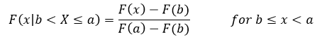
Notice we are looking at the limits that is because the integral only cares about the limits. Now we’ve fully defined our function! WOOO! But wait, we can find the pdf still, if we take the derivative like we did before we find that our pdf looks like this

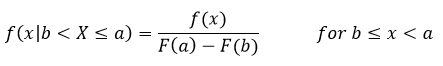
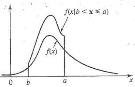
This result comes about because we only have one value where we can integrate and solve for x everything else isn’t dependent on x since it’s the limit. In any case this is bounded by the same limits so it is going to be zero elsewhere. This might be easier to see if we look at the plot of f(x|b < X ≤ a) and f(x) which come out to be

Why yes this is from my book since the internet was no help, why do you ask? (Still mad if you can’t tell)

And there it is!

Well we should probably talk about it a bit. All this math to tell you this, when we have a conditional pdf there is going to be an increase in probability density where the conditional holds in this case we said that P(A|B) happens between the values b and a, so those are the bounds and we see a proponal gain in the pdf (and therefore the CDF) when we are inside those bounds and zero when we are outside of those bounds.

Now you may be wondering why zero outside of those bounds? Well we are saying we are interested in the P(A|B) or the probability of A given B happened, if B hasn’t happened, then the probability of A is by definition going to be zero because we are conditioning it to the event B. In other words, if B hasn’t happened then the probability of A occurring when B has occurred is zero because B has not occurred yet. A simple example, P(heads|tails) what is the probability of heads given we had a tails on the previous flip? Well, if we haven’t flipped the coin even once, then the answer is zero, see?

Okay, well that was … a lot. Even for me and my usual long posts that was long. However, we are almost caught up to where I am and that is a good thing (for me anyway). Next up we can dive into functions of random variables. Yep, it gets even more complex, but hey we’re in this together.

Until next time, don’t stop learning!

*My dear readers, please remember that I make no claim to the accuracy of this information; some of it might be wrong. I’m learning, which is why I’m writing these posts and if you’re reading this then I am assuming you are trying to learn too. My plea to you is this, if you see something that is not correct, or if you want to expand on something, do it. Let’s learn together!!