Day 29: Probability density functions, Part 3

Don’t be scared, we’re going to tackle this guy today!

Well, apparently you guys really appreciated my probability density function posts. It’s good to see people interested in something a little less well-known (at least to me). So for those of you just joining us, you’ll want to start at part 1 here. For those of you who are keeping up with the posts, let’s review and then look at specific functions. Namely let’s start by going back to our gaussian distribution function and talk about what’s going on with that whole mess. It will be fun, so let’s do it!*

Okay, so yesterday we took a bit of a detour to talk about cumulative distribution functions. We said that our C.D.F. was just the integral of our p.d.f. from two points we are interested in, IE what is the likelihood that as X=x we will find a value between 0 and 1 or between 0.5 and 0.75. Then we thoroughly pimped out 3blue1brown because they did an amazing job breaking down calculus. We also said it was meaningless to ask what the likelihood is that we will find X=x at a specific value because we are dealing with continuous variables so if we said what is the probability that x = 3.2354235342 the answer would be zero because there are literally an infinite number of other values it could be.

There were a few other things we talked about, namely that different processes have different p.d.f. and that we can model quite a few of them as the gaussian (which is odd nature would do that, but still pretty wonderful). Then we discussed what the properties of a C.D.F. are, which you can read from our last post that was linked to earlier.

Okay, all caught up. Now let’s talk the gaussian. For those who need a refresher, that p.d.f. looks like this guy:

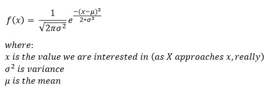
Yes, scary… but really when we look real hard and squint a bit we see that you only REALLY need to know the function and two things about the process we are modeling, that would be the mean and either the standard deviation or the variance (notice variance is the square of the standard deviation so knowing one gives you the other). This makes the function super handy!

So… now for the big reveal! If this is the p.d.f. how the heck do we integrate to get the C.D.F? Well the answer is, we really don’t. The problem is that this integrates into a big mess that can’t be written out in a closed form solution (IE without keeping an integral in the mix). Let’s take a look at the solution and discuss why it’s still a great tool.

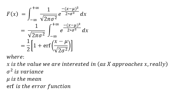
Okay, lots of math, but let’s take this one step at a time. So we integrate across the entire range of the function from -∞ to +∞. In the second step we pull out our constants, notice none of these involve our x which is what is changing across the range we are interested in (in this case we are integrating from -∞ to +∞ so all possible numbers). Then with some hand waving we derive the C.D.F. for the gaussian function. Notice this introduced a whole new function erf which is also called the error function.

The erf function is an important addition here, it has the values erf(0) = 0 and erf(∞) = 1. It also can be integrated, but please don’t make me write all that out. In fact, you can read more about the erf function here. Let’s look at a plot of the error function itself and you may see why this is important.

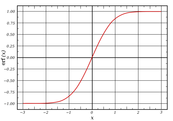
You may notice this look like something we’ve seen before, in fact this is just the error function, what does the C.D.F. for the gaussian distribution look like, well I’m glad you asked:

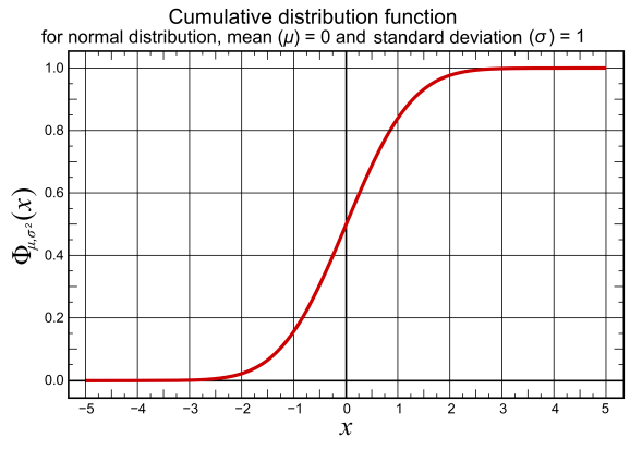
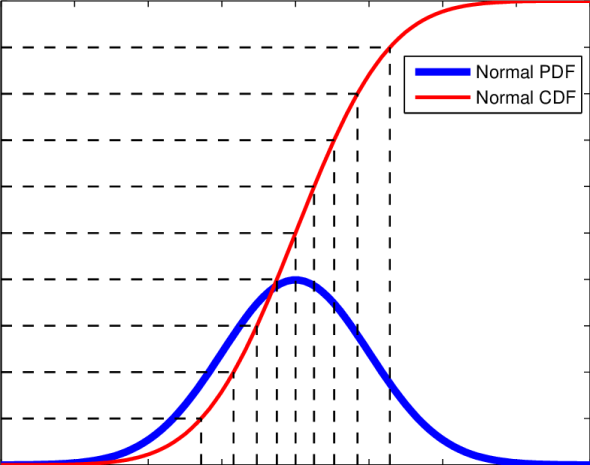
See, so at the heart of our C.D.F. is this so-called error function. All our particular C.D.F. does is shift it and stretch it (depending on the mean and standard deviation). Okay, but why does the C.D.F. always increase? We touched on this yesterday, but I find that visual demonstrations are best, so let’s look at the C.D.F. and the p.d.f. in the same plot and aligned to one another.

This is where we tie it all together. The blue line (the normally distributed line) is our pdf and our CDF is just the integration of our pdf. If we integrate the entire pdf our CDF will always be 1, but as we slide across the pdf we are looking at the probability that our x value is between -∞ and x, where x is represented by the dashed line. The point where the line intersects with the function (either the CDF or pdf) is the value corresponding to that function. If we look directly at the center of the pdf for example, we should have a value of 0.5 or 50%, following the line up to the CDF we see that it is about center to the function. This should make sense since we are looking at values of x for exactly half of the possible outcomes and it is centered around that point so we know that we have exactly 50% of the outcomes.

Now, keep in mind that we picked the 50% point for convenience of this example, not all pdf are going to be normally distributed so the halfway point between -∞ and +∞ isn’t always going to return a 50% chance of finding x≤ that halfway point (whatever that may be, it doesn’t have to be zero keep in mind!)

So this seems like a good place to call it a post. We’ve introduced the error function (erf) and talked about why it is important to our CDF, we’ve looked at our pdf and CDF and showed how one relates to the other, and we looked at some examples of this. We covered a lot, don’t worry if you’re not getting everything, it will hopefully make sense as we continue to look at more and more examples!

Until next time, don’t stop learning!

*My amazing readers, please remember that I make no claim to the accuracy of this information; some of it might be wrong. I’m learning, which is why I’m writing these posts and if you’re reading this then I am assuming you are trying to learn too. My plea to you is this, if you see something that is not correct, or if you want to expand on something, do it. Let’s learn together!!