Day 28: Cumulative Distribution Functions

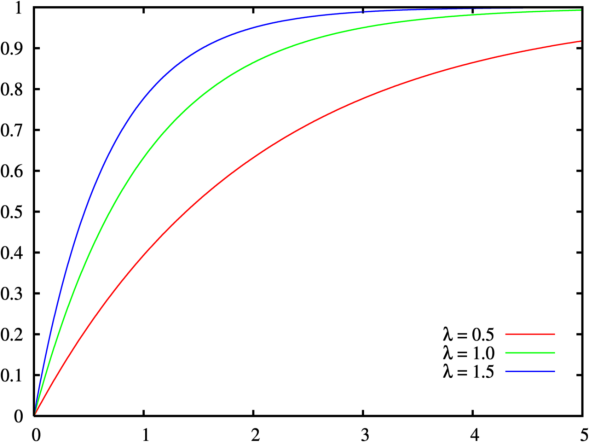
An example C.D.F. of an exponential distribution

Today we were going to do another deep dive into the p.d.f and C.D.F. relationship. Specifically today we were going to talk about specific p.d.f. functions and why we use them, however… I am not doing so hot today, so instead we are going to back track just a bit and talk about what how a C.D.F. differs from our p.d.f. even though we kind of covered it, it would be nice to be clear and I can do this in a (fairly) short post for the day. So that said, let’s get started and we will pick up our p.d.f. discussion next time (maybe).*

When we deal with continuous variables like we have been the past two days, we can convert our p.d.f. into a C.D.F. by taking the integral of the corresponding p.d.f. In practice you can get a C.D.F. for discrete cases if the values of the random variable are ordered, but that is a whole other topic. If you look at the cover image for yesterday’s talk, you see a p.d.f. (wrongly labeled as P.D.F. and I’m sorry for that, this is why we are using the C.D.F. notation for our discussion, it makes it slightly less confusing) and the corresponding C.D.F.

You’ll notice a few things that are important to cover. First is that the peak of our C.D.F. reaches 1 (eventually) and stays there. This should make sense because it would be nonsensical to have a probability higher than 1, which corresponds to 100%.

There are a few important properties to know about your CDF functions, one is that it is nondecreasing. Yep, the probability that an event will occur increases as you get closer to the edges of the entire probability space. For an example say we have the function from yesterday:

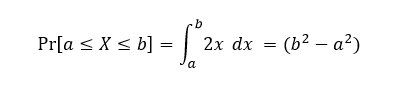
Which we said X ranged from a value of 0 ≤ X ≤ 1, and the range we were interested in was set by our a and b (IE from 0.25 to 0.5 or 0.75 to 1). What this rule says is that the closer we get to a = zero and b = one when asking what our value X is, the more likely we will hit 100% because we’ve covered the entire range of probabilities. Each probability function has its own associated C.D.F which is found by taking the integral of the p.d.f. like shown above. Again, if you want an introduction to calculus I cannot recommend enough 3BLUE1BROWN, I’ve watched the entire section multiple times and I always walk away with a better understanding of calculus. This coming from the guy with a masters in mechanical engineering, so I highly, HIGHLY recommend a review. In any case, enough pimping other people’s work.

Also important to note, our function is always right-continuous. This is just a fancy way of saying that if we take the limit to some point c, no jump in values will occur when coming from the right (not true coming from the left however!). We can cover why this is important later, but I wanted to give some introduction to the C.D.F. since we will be talking a lot about it over the next few days (or more).

Okay, I did my best everyone. I’ll be back tomorrow with some more. This seems like a good (albeit short) introduction to the concept of the C.D.F in a more explicit sense. We will look at what a right-continuous function means exactly and look at how we use the p.d.f. and C.D.F. in statistics some other time. But for now, we’ve introduced some of the properties of C.D.F. and we will be building on this in the future, so it was important to cover.

Until next time, don’t stop learning!

*My amazing readers, please remember that I make no claim to the accuracy of this information; some of it might be wrong. I’m learning, which is why I’m writing these posts and if you’re reading this then I am assuming you are trying to learn too. My plea to you is this, if you see something that is not correct, or if you want to expand on something, do it. Let’s learn together!!