Day 32: The Laplace pdf

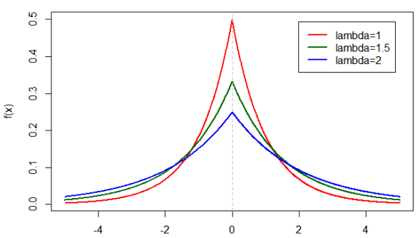
The laplace p.d.f with a θ = 0.

Well here we are again… maybe unless you’re new, in which case welcome. If you are just joining us we are talking p.d.f. no not the file format, the probability density function version. If you’re new, you may want to start back here(ish) If not, then let’s talk the strangely similar laplace distribution.*

If you recall from our last post we introduced a somewhat simpler distribution function (at least compared to the gaussian distribution). We talked about what it was used for and originally we had planned to look at some examples. Instead however, today we should touch on the laplace distribution while the exponential distribution is still fresh in our memory and we can go over some examples of both at another time. After all, we aren’t even 10% of the way done with 365DoA, so we have time.

If you notice I keep alluding to the idea that the exponential distribution is similar to this new laplace distribution we are talking about, and it is. In fact it really is the same distribution reduced by 1/2 and mirrored along some value θ. Since we’ve started breaking more into the math regarding these concepts, let me show you what I mean. The laplace pdf looks like this guy:

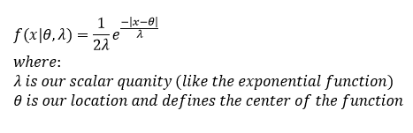
One important thing to note is that λ has to be greater than zero. Our θ (really the mean of the function) has no constraint and can be any value we want. Additionally, unlike the exponential function, our x has no limitations on it now, it can be any value from – ∞  ≤ x  ≤ + ∞. This is because (if you noticed) there are only two things different from our exponential function. One of them is the 1/2 value added, the second is that we are now taking the absolute value of our x-θ so no matter what we are always going to have a positive output (prior to the added negative sign).

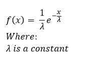
Okay, well we’ve compared this to the exponential function, but let’s put the exponential function here so we can compare on the same page. The exponential pdf looks like this guy from yesterday:

Notice that we had an extra value in the new function θ, this just shifts the zero point left or right along the x-axis and has no real impact on the look of the function itself. Now you may be wondering at this point if our C.D.F. looks the same or not, well it does look slightly different, but that is just because we are now dealing with two different parts of our function, we can have two separate cases now. In one case x ≤ θ and in the second case x > θ, so here we need to integrate across the two different conditions to find our new C.D.F. While this is a little complex, specifically for those who haven’t taken calculus classes, we will walk through it together and when we are done we will see that there are two different C.D.F. one for each of the two cases we just created. Let’s take it step by step:

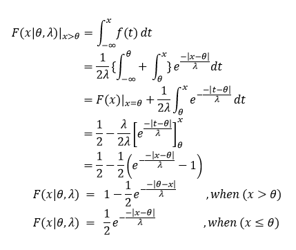
Okay, we derived the CDF (for one case and I gave it for the second to save some time and space). We can see some interesting things if we look at our functions, when x ≤ θ you’ll notice that our function is increasing in value, when x > θ we are moving from a maximum and decreasing, so the likelihood of finding a value as we move away from θ decreases in either direction. The plot at the top of the page shows what the p.d.f. looks like, remember that by definition our C.D.F. is always increasing, so while the probability that we will find our value as x moves away from θ (our mean) decreases in the pdf, as we move along the x axis, we gain probability that we will find our value between – ∞ and x. Actually, we can plot the C.D.F. to show you what I mean:

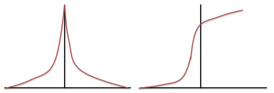
Our laplace p.d.f. (on the left) and our always increasing laplace C.D.F. (on the right).

Yes, it is a little tricky to think about, but remember as you move towards θ coming from – ∞ the probability increases so you get a rather large increase in the CDF before you hit the mean, then it slowly keeps increasing because you are still adding probability mass to the function (because we are looking from – ∞ to x as x goes to +∞). This is why the value always increases, because you are including all previous values as x increases (remember we are dealing with the area under the curve, which in this case is always going to be positive).

For now, this seems like a good place to stop. You can probably see why I wanted to cover this while it was fresh. Next we can look at some examples of how we can use these functions are used and why we would use them in the first place.

Until next time, don’t stop learning!

*My dear readers, please remember that I make no claim to the accuracy of this information; some of it might be wrong. I’m learning, which is why I’m writing these posts and if you’re reading this then I am assuming you are trying to learn too. My plea to you is this, if you see something that is not correct, or if you want to expand on something, do it. Let’s learn together!!