Day 33: Example of the Exponential pdf

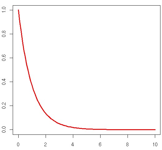
For those who need a refresher, this is a plot of the exponential pdf we are working with today.

Over the past couple of days, I’ve been talking about several different types of pdf and the associated C.D.F. Hopefully, we have a clear understanding of each of those concepts, for those of you scratching your head, I would recommend you start here at this other post. Otherwise, let’s (finally) look at a real life example using the exponential pdf!*

Okay, so we touched on a lot of things the past couple of posts, but in particular the last two had a lot in common. We will see an example of the laplace pdf in another post, but today it seems like a good idea to go over at least one example of how we use a pdf in real life. Thankfully the exponential distribution is a perfect way to show a real world application, mostly because it is based on real world events. Let’s take a look at what I mean by that.

If you recall from our exponential pdf post I showed two ways to write the pdf, one way made it really easy to see the relationship between the exponential and laplace pdf’s, but we also hinted at the use case for the exponential pdf in the process. We said that the exponential pdf was used to model the time before a random process occurred. If I recall correctly, we used a bank example.

There are other ways to use the exponential pdf, namely product reliability. However, it also can be used for other purposes, like our bank example, or other wait time models. We can use this pdf to answer questions like, “How long before a hurricane hits,” or “How long until my car breaks down.” Let’s look at an example explicitly though so we know what we are dealing with.

Let’s go back to our bank example and work it out exactly. Let’s say that, on average, we have 50 customers that arrive per hour. This means that our mean interval between events (the time between one customer to another) can be said to be

50 customers / 60 minutes = 0.8333 customers per minute

Not a nice round number, but that’s what we get for coming up with an example off the top of my head. This just means that on average (again average) we would expect a customer to come into the bank every 0.83 minutes, or every 50 seconds. It’s a busy bank!

Okay now let’s look at our equation and see how this fits into it.

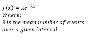
If  λ is our mean number of events over a given interval, then that is what we just calculated. We just determined that our  λ = 0.83. Now, let x = T, because we are explicitly dealing with time, in this case because units matter we are dealing with minutes, said another way x = T where T is time in minutes. Now we want to find out what the probability is that a customer will come into the bank in the next 30 seconds or 0.5 minute? In this case we say that P(T≤ 0.5) which we then integrate over our interested range of time (to find our CDF), then plug in the values. Let’s do that:

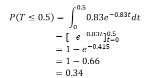
Okay, so the chances that a customer will come in in the next 30 seconds is 0.34, that may seem a little low considering the rate at which customers come in, but remember that on average a customer only comes in every 50 seconds, so we still have a full 20 seconds before we’ve even managed to hit the average. Now let’s say we were interested in finding the probability that a customer will come in after 90 seconds or 1.5 minutes, this should give us a higher probability, but let’s see what the CDF says:

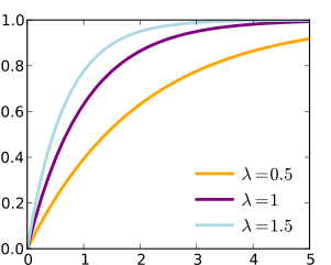
This gives us a much, much higher probability that someone will come in within 1.5 minutes. Two things we should keep in mind, as time T approaches +∞ our probability P(T) will approach 1, so the fact we don’t get a 100% chance someone will come into the bank makes sense in that aspect because the mean is just the average value, you may have 2 or 3 people come in at the same time. The second thing is that as T approaches +∞ the probability someone will enter the bank increases, but that increase becomes less and less. This also makes sense if we look at the pdf at the top of the page we see that it decays and the C.D.F. is just the area under the curve, so the chances of an event occurring are going to increase at a faster rate the closer we are to our start time, but this behavior is dependent on our λ value. Let’s look at the general C.D.F. to show you what we mean by that:

Until next time, don’t stop learning!

*My dear readers, please remember that I make no claim to the accuracy of this information; some of it might be wrong. I’m learning, which is why I’m writing these posts and if you’re reading this then I am assuming you are trying to learn too. My plea to you is this, if you see something that is not correct, or if you want to expand on something, do it. Let’s learn together!!