Day 48: Functions of One Random Variable Example Part 4

A simpler example than yesterday.

Still feeling under the weather, but the show must go on as they say. So today let’s look at another example of how to solve functions of one random variable. Today will be another shorter post, but as usual I’ll try to explain everything step by step and hopefully you’ll see the methodology behind solving these types of problems.*

As usual, if you are just joining us and are learning about functions of one random variable, you should start here at the beginning of this section of posts. This will be our forth example of one of these types of problems and by now I hope that some of this is making sense. I’m sure that some of it may be harder to see than other parts (specifically the derivation and integration if you aren’t familiar with it and in some cases even if you are), but I’m hoping that the overall effect is positive. So let’s get started.

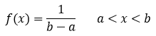
Let’s say that we have X which is a continuous random variable with a pdf where X ~Uniform(-1,1) and

Now you may recall that we did an example with the same function, but after some thought I figured it would be good to do another example with something a little simpler. So let’s find the CDF and pdf of Y. So if the last post was confusing, my advice would be to let’s do this and then go back and see if it makes any more sense to you.

First thing we need to do is see that because we are squaring X we can ignore the negative values (because the square of any real number is positive). So our limits for our new function become

for

This next bit should seem familiar since we’ve done this before, but we plug the function of our random variable in, redefine the limits in terms of our X and solve. Let’s see what that looks like

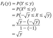
Now, like we just said, plug in our function (step 2) then redefine the limits in terms of our original X function (so square root) and remember that the square root of a square gives a positive and negative value so we have our upper and lower bounds now (step 3). Now we plug in our values and solve, now remember that our normal distribution CDF looks like this

and we noted that our function was a uniform function where X ~ uniform(-1, 1) so a = -1 and b = 1 and we set x to our squareroot y value (step 4) and solve (step 5) 1-(-1) is 2 and squareroot(y) – (- squareroot(y) is just 2*squareroot(y) so we are left with our solution (again step 5). Therefore our CDF of Y looks like this

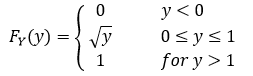
Now we have the CDF, finding the pdf should be pretty easy at this point (we’ve already defined our range of integration and we have our function, so we integrate and find

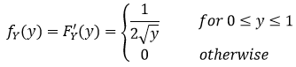
I’ll leave you to do the integration yourself to see that this is the solution. What? I don’t feel well, so I’m being somewhat lazy. In any case, like I mentioned at the start of this, this should be an easier example to grap than our example yesterday so hopefully it clears some things up. When I’m feeling better we can do some other things, but for now reviewing is as good as learning something new anyway.

Until next time, don’t stop learning!

*My dear readers, please remember that I make no claim to the accuracy of this information; some of it might be wrong. I’m learning, which is why I’m writing these posts and if you’re reading this then I am assuming you are trying to learn too. My plea to you is this, if you see something that is not correct, or if you want to expand on something, do it. Let’s learn together!!