Day 49: Functions of One Random Variable Example Part 5

Let’s look at something a bit different today!

If you’ve been following along, we’ve been taking it easy the past few days. I’ve also been going over (relatively) simple examples, so today we’re going to take a more complicated example and work through solving it. I may go over a few more examples to be honest, only because this is important to what comes next, after we nail this down, we’re going to get into functions of two random variables and as you can imagine that’s a little more complicated (a lot more).*

Just a reminder, we’re pretty far in the mix here, so if you’re just joining us, you may want to start at the beginning. The last two examples used the same function of X (our Y function). Today instead of just squaring our X value, let’s say that we don’t even know our X function.

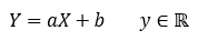
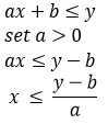
Now, let’s say that our Y function is y = ax+b. If we want to solve this we need to find the values of x such that ax+b ≤ y. This should look familiar since we’ve done something similar in the past, but in this case we still don’t know X, so how do we solve this? Well first let’s look at it in math terms. If a > 0, then ax+b ≤ y for x ≤ (y-b)/a. How do we know that? Well let’s look at the steps

we’re just rewriting the information we were given to determine something about one of the variables. So now we can plug some of this into our equation (the probability one we have been using) like this

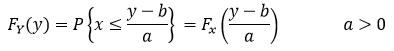
Without knowing what our X function is, we’ve already determined a limit for our Y function. You may have noticed, but really we are solving this backwards, we know Y and we are trying to learn something about X.

Now that we have this first limit you may know what’s coming based on our other examples. It’s time to find out what happens when a < 0. In this case we still have our equation saying ax+b ≤ y, so

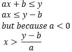
notice that we flipped the inequality, this is because a < 0 so ax < y-b because a is making x negative (a < 0). Now we can plug that in like we’ve done in the past and say that:

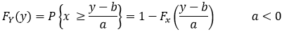
and without knowing anything about X we’ve solved as far as we can go, but if you notice the two functions we found describe the function fully, we just don’t know the behavior of our random variable X, so we cannot go further. Also notice that our a < 0 equation is just one minus our a > 0 equation, this isn’t an accident, if you think about it this should make sense we’ve solved up to a > 0 and when a < 0 the value is just whatever is left up to that point (since we are talking CDF here so it MUST sum to 1, always, no exceptions. In fact, an easy way to check your work is make sure your CDF sums to 1 by plugging in the maximum values.

Until next time, don’t stop learning!

*My dear readers, please remember that I make no claim to the accuracy of this information; some of it might be wrong. I’m learning, which is why I’m writing these posts and if you’re reading this then I am assuming you are trying to learn too. My plea to you is this, if you see something that is not correct, or if you want to expand on something, do it. Let’s learn together!!