Day 51: Joint Cumulative Distribution Function

As promised, today we are going to talk about two random variables that are not independent. This means that the individual probabilities don’t sum to be equal to the joint probability (like they did yesterday). Like our normal CDF, we can find a CDF for two random variables, but let’s take a look at how this works.*

First we are going to have to define a few things if we are going to talk about a joint CDF. When we talk about a joint CDF of two random variables (which is sort of redundant, but it’s nice to be clear). We can write our CDF so that:

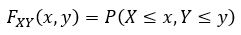
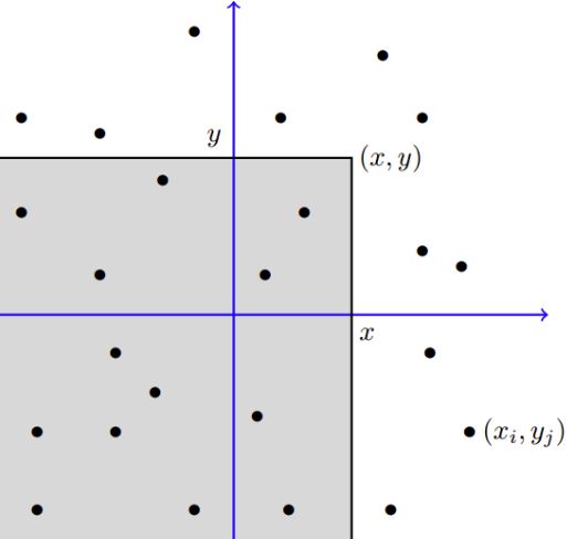
Where the comma simply means “and.” So when we talk about CDF you can think of it as a single dimension (a line). We haven’t really introduced this type of thinking, but it will help going forward. So when we are going from a sample space to a pdf we are converting one dataset to another form. In this case, we have two variables, so we have a two dimensional space that we are working in. So what is the probability that X and Y will be in a certain area, well to visualize it, you would see something like this

Where the shaded region would be our region of interest and individual x and y values would fall into this total space. Note however that we are only showing a few solutions (dots) because really it could fall anywhere in the region if it is continuous, but this way of showing it is (hopefully) better to give you a visual idea of how this works. Also note that we extended our range from – ∞ to x and from  ∞ to y, we don’t need to do this, we can specify an actual box that we are interested in of size a to b and c to d in the x and y plane respectively.

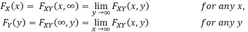
Now, solving these can be difficult, so we can solve for just one variable at a time. This is called the marginal. We solve for the marginal CDFs like so, say we are interested in finding a value x, we would set the y value to be the entire space, from -∞ to +∞ like so

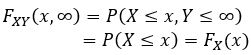
this would be the marginal CDF for our X value, we can do the same for our y by setting x to infinity, which looks like this

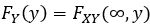
And when we solve for the marginals you may see it written like this:

Finally, let’s look at some basic properties of joint CDF’s with respect to the marginals

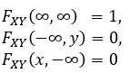
For the first one, we are looking at the entire space, so the probability is going to be 1. That should be fairly easy to see (specifically because we are looking at every possible outcome so the odds of anything happening is going to be 1). The other two are a little more difficult to see right away, we are saying that if we set either value (x or y) to the minimum value, the odds of anything happening are 0. Basically what we are saying is what are the odds something will happen at a specific value along the x or y, which as we know from before will always be 0, same thing in this case.

Tomorrow we can look at an example of solving one of these joint probability models, but for now this looks like a good place to leave off.

Until next time, don’t stop learning!

*My dear readers, please remember that I make no claim to the accuracy of this information; some of it might be wrong. I’m learning, which is why I’m writing these posts and if you’re reading this then I am assuming you are trying to learn too. My plea to you is this, if you see something that is not correct, or if you want to expand on something, do it. Let’s learn together!!