Day 52: Joint Cumulative Distribution Function Example 1

We’re getting into some interesting things today!

Well here we are again, today we are talking functions of two random variables. If you’re looking for the beginning, this isn’t it, but you can read the introduction here. If you’ve kept up, then you’re ready to go over the example we have today, so let’s get started.*

Let’s do a quick review of how we got here. First we introduced the idea of random variables. It’s been a while since those days, but next we introduced functions of random variables. After that, we went through a few example and now we find ourselves looking at two random variables (not functions of two random variables, but we will be covering that soon).

Now that we are up to speed, let’s take a look at an example of two random variables. Now this won’t be our first example, we did that here. However, this will be slightly more complex. The previous example and this example will both be using independent random variables, we can look at dependent examples soon, but we should go over at least one more example before we start diving into more complex examples.

Okay, now let’s say that we have two random variables X and Y. Let X ~ Bernoulli(p) and Y ~ Bernoulli(q) where both X and Y are independent. We will also say that 0 < p and q < 1. Now let’s find the joint p.d.f. and CDF for X and Y.

First let’s look at the range of X and Y, based on what we were given we know that

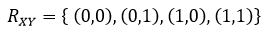
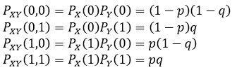
also, remember that we said the random variables X and Y were independent, meaning we are really dealing with two single variable equations multiplied together, in other words

So just from that, we can plug in our values and find a solution (which is why we are starting with a simple example). So we have four different possibilities, and therefore have four different equations like this

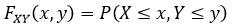
However, this is just our pdf, we also want to find our CDF and we do that the same way we’ve done the other examples, by saying

Next we find the limits of our function like we did for the pdf, since we know that 0 ≤ X, Y ≤ 1 we also know that

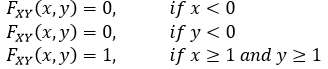
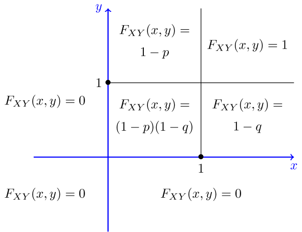
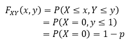
So three cases, and three solutions. Now we just need to find the in between bit (like we’ve done previously). First let’s look at the case when 0 ≤ x < 1 and y ≥ 1 for that case we have

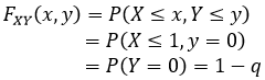
Now let’s look at the case when 0 ≤ y < 1 and x ≥ 1, in that case

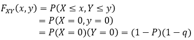
Lastly we need to look at the case where 0 ≤ x < 1 and 0 ≤ y < 1, when we plug in those values we find

So basically the same solution steps we use when we solve these types of equations and you’ll see something similar when we go onto dependent variables. If you look at the plot at the top, you’ll see where each of these cases fall. Something to remember, these types of problems usually are in three-dimensional space, however we used bernoulli so we could collapse the example to two-dimensions.

Next up, dependent variables! However, getting into that means adding complexity, so hopefully the example today helps clarify some of the solving process for at least this case where the two variables are independent.

Until next time, don’t stop learning!

*My dear readers, please remember that I make no claim to the accuracy of this information; some of it might be wrong. I’m learning, which is why I’m writing these posts and if you’re reading this then I am assuming you are trying to learn too. My plea to you is this, if you see something that is not correct, or if you want to expand on something, do it. Let’s learn together!!