Intro to ICA

Independent component analysis, probably not something you hear about all that often unless you’re in a field that uses it. If you’ve found this via google or the such, then you’re probably looking for an explanation on what the heck ICA is and how to use it. Fear not, today we’re going over the why of ICA, why it works, why we use it, and why it isn’t the perfect tool we wish it was. Hint, the reason it isn’t perfect is because of math, stupid math. Quick note, I’ll be focusing on EEG uses for ICA, but there are tons of other applications and this knowledge will still apply to them as well.

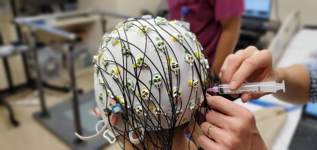
Today I taught a class on independent component analysis or ICA for short and since I like sharing today we’re going over the content here. ICA is a way to separate out signals that are mixed together. Say you’re at a bar and it’s packed, you can’t hear the person next to you it’s so loud. Now imagine we surrounded the outside of the building with microphones. Could you believe that we could extract useful information from those microphones? That’s where ICA comes in for my purposes anyway.

In my example the people talking would be neurons, the bar would be your head and the microphones would be the EEG electrodes. Signals recorded from the brain aren’t going to be a single source, at least not when we record them non-invasively. It’s a combination of a whole bunch of activity all going on at once, just like the bar example. The “sources” are the people talking and in the brain that would be hundreds of thousands of neurons firing together. We think they fire together and sync up because they are weakly interacting (here’s an example with metronomes), which is why we can record activity from the brain non-invasively at all (more on that here).

The issue is that other clumps of neurons are firing and syncing while we’re recording so we have groups of neurons firing at different rates and doing different things at the same time. This causes our recordings to be a linear combination of the sources. Sort of like at a bar you can more easily hear the people closest to you, but you can still hear the people across the bar, if only barely. The same thing happens in the brain so when we record with EEG you get something like below. In this example we have two sources and in this imaginary example we know exactly what the sources are doing, but the recordings from the sensors are mixes of the two sources and depending on the sensors we have different amounts of each source coming through.

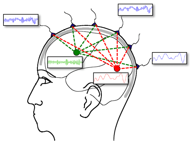
Of course in the brain there are going to be far more than two sources, but sometimes simplifying helps. You’ll notice in our example the closer the sensor is to the source the more that source can be seen, but even the sensors closest to our sources are still contaminated slightly with the other source. This is where ICA comes in, we can use ICA to get back to our source space from what we call sensor space. Let’s look at how that works.

First we need to understand what we mean when we say independent. Independence is a strong word in statistics and to have independence we say that the two events are unrelated (that is the probability of A occurring after B has occurred is just P(A)P(B) which is important). When we’re dealing with ICA it helps to understand PCA or principle component analysis because they do similar things. PCA is used to find uncorrelated sources, being uncorrelated does not mean they are independent, but independence means they are uncorrelated, sort of like there’s water in a river, but water does not always mean you’re dealing with a river.

We actually use PCA in ICA because it makes things less computationally intensive, but I won’t get into that too much, instead let’s look at a 2 dimensional example. Say I have two EEG electrodes or microphones, or however you want to think about it, it’s all the same. We can plot the output from one microphone on the x axis and the other output on the y axis (think of our output for both as amplitude so it makes sense to plot them like this).

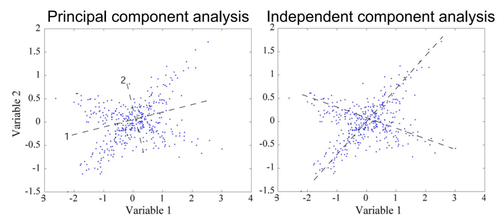
All PCA and ICA do is try to rearrange our x and y axis to get something out of the data. In PCA we’re looking for dimensionality reduction. Axis 1 does a better job of describing the data than our x-axis does because the data fit a wider range on axis 1 then on our x axis or our y axis. This maximizes our uncorrelatedness meaning I cannot tell what variable 2 was doing just by knowing the value of variable 1. This sounds bad, but it’s useful because if I could tell variable 2 from variable 1 perfectly then I don’t need variable 2 at all. I know what variable 2 is doing with variable 1 alone, so we’re maximizing information content of our two variables!

ICA on the other hand separates our data into independent components, notice how both are really just ways to transform our coordinate system. Keep in mind this is easy to visualize in 2 dimensions, but when working with high density EEG we have 60 or more dimensions and you cannot visualize that! It helps if I draw what our components look like so below I’ve highlighted how both transformations work.

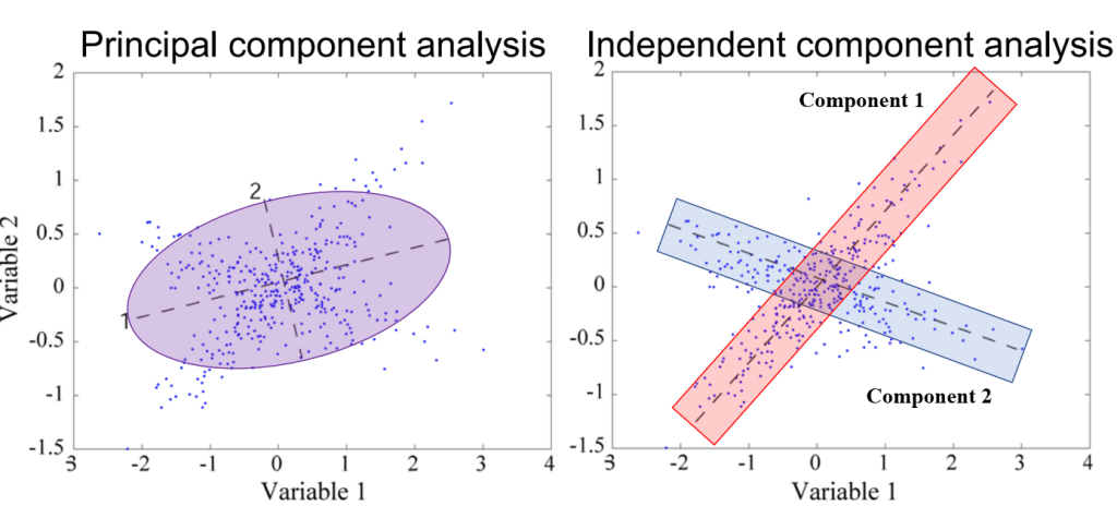
ICA breaks our data into components so it would return the values of component 1 and component 2 and those would be our two IC’s. There are a few things to clarify though. First, ICA is blind source separation so it doesn’t need to know where the sensor is located, this is good because it makes it flexible. We can use sensor location to triangulate the location of the source within a reasonable margin (called dipole fitting), which we can discuss some other time maybe. Second, ICA doesn’t care about time, so the longer you’re data are the better, but time doesn’t matter here. Third, the technique will return at most 1 IC per sensor, you can see why above, in 20 dimensional data we have 20 sensors and we can only arrange 20 axes in our data so we get 20 back AT MOST!!

Now for the why this isn’t perfect. If you look above the red box of component 1 and the blue box of component 2 overlap. That’s the problem. Seriously and that’s why I like visualizing the data like this. The issue that part of component 1 is now grouped with component 2 and vice versa. This means you can’t have a pure IC no matter how hard we try (wahh!!). That isn’t to say we can’t get close enough that it doesn’t matter, because we do and we use this technique because more often than not it doesn’t matter. The issue is that sometimes we need to make hard choices to eliminate a component because it has significant amounts of noise, even if the component also has useful data.

There is one other thing I should point out. We can go from sensor to source space and back again, but in source space our sources (components) are unitless, the units sit with the weighting matrix, which we’re about to cover. The second is we can’t actually determine amplitudes anymore. Things will get scaled, so all the data will be the same for our purposes, but the amplitudes will be different. It’s not a huge deal since the scaling is uniform, but it’s something to keep in mind.

Now for the math behind all this. Going from sensor to source space we need to whiten our data or sphere it. This means we find the minimal amount of correlation and that’s done using PCA (mostly)! Hence why we covered it, then ICA draws our new coordinates in our data and we do that using something called a weighting matrix (sometimes called a mixing matrix, but I prefer weighting matrix so that’s what we’re using here). That’s just the first step, but for that step our math looks something like this

W = weights × sphering matrix

Where W is a n by n matrix and n is the number of sensors you used. I will not be covering the math to get these matrices explicitly, but I do want to cover what they mean and why we use them. The math would make this incredibly long and probably not as useful. If we let our EEG data be called x then our transformation from sensor space to source space is just “simple” multiplication,

a = W*x

where a is activations and how this is commonly written out, but you can just think of it as our sources. In source space we can remove sources that are noise then return to sensor space to do any sort of analysis we want (or you can work in source space too, that’s up to you). To go back we just take the inverse of our weighting matrix W and multiply it with a or for those math inclined

x_clean = a*inv(W)

where inv(W) is the inverse of W. Notice that no matter how many IC’s I remove I will always get back the same number of sensors I started with because W is always going to remain the same size. So if I had 60 sensors and 60 IC’s, but removed all but a single IC I would still get 60 channels worth of data when I go back to sensor space, but the data would be significantly changed. Below is a good graphic of what all this looks like

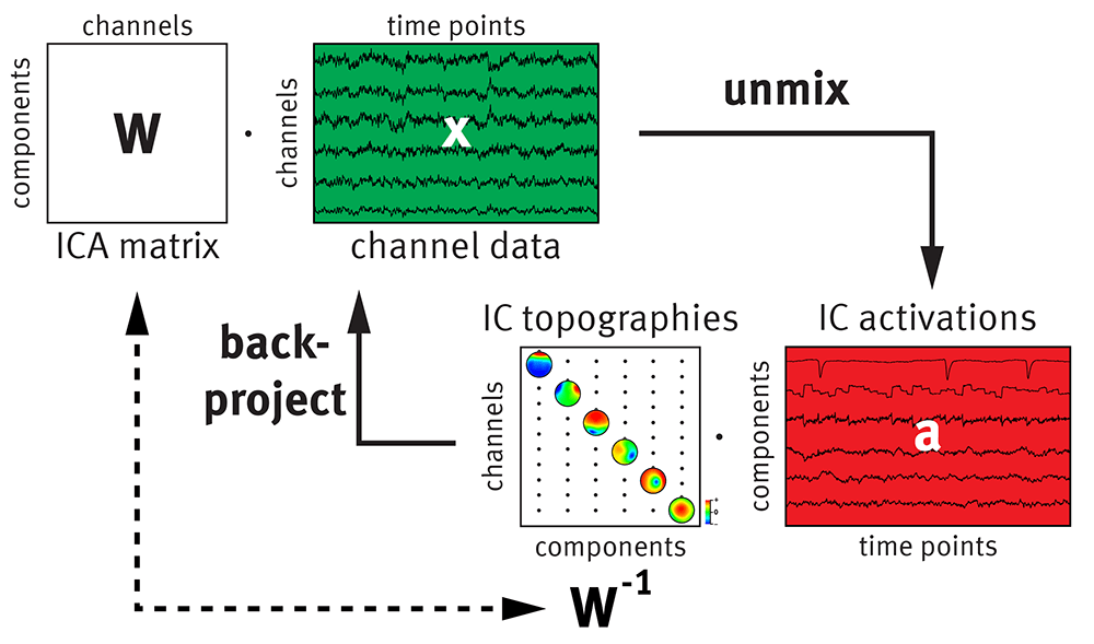
In this case our IC topographies are the inverse W and when we use our sensor locations (like above) we can plot which sensors most contribute to that IC. Keep in mind that even though our IC is a single channel, it’s made up of contributions from all n sensors. The inverse weighting matrix tells us those contributions and by knowing the sensor locations we can locate the source in the brain (somewhat by looking at the IC plots, but mostly using dipole fitting).

Now I’ve covered using ICA for EEG data, but you could use it for just about anything. Want to isolate the drums in a recording of music? ICA can do that for you. I mean there are a lot of different applications outside of EEG, but since my application is EEG, that was the focus of this writing. Keep in mind that this is a high level overview of what ICA is, does, and how we use it. It’s not all encompassing, but I think for an introduction it’s more than enough to get you started.

If you’re using ICA for cleaning EEG data artifacts, you’re basically using pattern recognition and there is software that will remove IC’s that are determined to be artifacts, but I prefer doing it by hand since there are a lot of things you need to consider going into this. If you are doing EEG cleaning and want to practice figuring out which IC’s are noise and which are good data I recommend this game which gives you a chance to practice and will let you compare what you selected with several other users and experts in the field.

Who knows in a future post I could go over how to tell artifact from brain signals, but for now let’s just call this good. As usual questions, comments, or thoughts are always welcome!