Intro to MATLAB – Part 1

Per my usual routine, I’m teaching a class and instead of hording the knowledge I’m putting it here for all of you to use! I’m even going to attach the example code I wrote, which has enough comments to fill a small book, to help everyone just starting out. As I explained to my students, this is an intro to MATLAB course so my focus is on showing how things are done in MATLAB and less on how to problem solve using MATLAB. Although the last two lectures have not been created yet so they may focus on problem solving, who knows.

For those just finding my blog or finding this post in particular, the story goes something like this a few days before the first class my main-PI came to me and told me I would be teaching this course. I’ve gotten really good at using MATLAB, so he wanted me to instruct some of our summer students on how to use it. There’s a whole post on how I got sucked into doing this class (here) for anyone wanting more of the backstory. With that let’s dive into what MATLAB looks like.

This first class I focused on orienting my students in the MATLAB software, so the basics where to find stuff, why things were listed in a particular way. How to change the color scheme even (there’s some handy code that will do it for you automatically). Below is what my MATLAB program looks like, the colors are different and the window organization is slightly different, but it’s still all the same thing.

I’ve created several colored squares to help us navigate what is what. For people who have trouble distinguishing the colors, I’ll walk you through where I’m talking about as well. Starting from the square in the top left (brown), we have the new script button. I highlight this for my students because I learned the hard way no matter what you do, no matter how “done” you think something is, you should always write a script for it. ALWAYS. If it’s more than a single line of code, write a script, save it, thank me later.

Now for the middle top box (the purple one), the box still on the tool bar. That’s the preferences menu and it takes you to a magical place that will let you adjust the colors manually (or again just use some code). There are a lot of other things in that menu that you can adjust. When you click the button a new window will pop up (seen below). I have the colors selected, but you can also adjust the fonts and things to make it easier to read.

There’s also a lot of other things that can be adjusted, but mostly I leave my settings the way it was when I installed the software. Instead I change the color and I do adjust the command history so I have access to more of the previous commands I entered. Normally it’s set to save the first 1000 commands or something along those lines (probably 10,000, but don’t quote me on that) I set it orders of magnitude higher because there are occasions where I will want something I entered into the command line for testing from a few months back and I can find it that way (you can also have it display the date and time the commands were entered which is super helpful in cases like that!

Now onto the other boxes, this one is the middle left of the photo of MATLAB (red). It’s probably hard to read the words unless you open the imagine in a new tab (hint), but that is our current folder. The current folder (or working directory) is the directory you’re using to run code. Right now all that is in that folder are the two code examples I’ve written for my class, but say I want to run the class1 code by using a command in the class2 code. As long as the code I’m trying to call is in the same directory MATLAB will find it. This is useful because often times I will write a bit of code that does something specific and I will write some new code that will “call” that code to run and MATLAB won’t search my computer for it unless I specify the directories I’m using. There is a way to add directories for MATLAB to search that are not the working directory and I’ll show that in a minute, but let’s go through the rest of the squares.

So middle of the screen, middle box (blue). The largest box and the largest portion of the screen is taken up by our command window. This is where I can manually type out code into the command line to test or to run. As I said before always, ALWAYS!!! write your code as a script so you can save it. The command line will keep a history, but you won’t be able to run it nicely again so organizing your working code in a script will save you so many headaches. I use the command line often. Mostly to test code before I add it to my script so say I want to write a code that will take one variable and add two to it, in my script it may look like this:

NewSum = OldSum+2;

The NewSum is my variable name and I’m setting it equal to my OldSum, which is a variable that already exists and can be anything in this case, then I’m adding 2 to it. The ; at the end of my code suppresses the output in the command line. This means when I run the code the command line wont show that I ran anything, which is useful because it turns into an ugly hard to read mess, but the code will run and it will update my variables.

Now say I wanted to make sure that the above code would run. Now it’s simple enough that I can trust it, but there are tricky bits of code you may want to test beforehand. I like to do that in the command line using something like:

tst = OldSum+2;

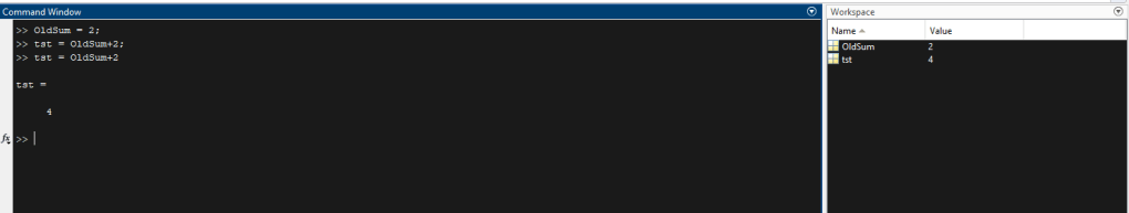
This will create a new variable tst and it will let me check to make sure that my output is what I expect it to be. If OldSum is equal to 2, I can check that tst = 4 in the next box we’re covering. On the far right middle (yellow) we have our workspace. Now this workspace is empty because I haven’t done anything yet, but the workspace will keep all the variables I’m using for that session. Meaning if I close MATLAB they all go away, they don’t get saved anywhere unless I specifically save them. Below I’ve created OldSum = 4; and tst = OldSum+2; then I ran tst = OldSum+2 (without the ; at the end of the command) to show that it will return the value of tst in the command line when you don’t suppress it. Notice my workspace now has two variables OldSum and tst and the values of each are listed. This is the case when your variables have a single value, but you can have vectors, matrices, things like that and the command line will only show you the size of the variable (so if a vector v is a row vector that has 20 numbers, the MATLAB will show it as a 1×20 or 1 row x 20 columns).

In fact, here’s the vector v example as seen in MATLAB workspace.

Our vector v is a 1×20 double. Double signifies the precision and double precision gives us 2^64 options for a number or roughly 9,223,372,036,854,775,807 ways we could create a number. That seems overkill, but that’s only thinking with whole numbers, we have decimals so when we have 0.001 for example we’ve suddenly added a few hundred different options and we’re still in single whole digits. Anyway MATLAB defaults using double precision, but on occasion a function will return single precision (2^32). You don’t need to really understand this other than in neuroengineering we try to stick with double precision and MATLAB will generally stick with double precision as well.

So now you’ve been introduced to the idea of a variable, a vector, and now we can talk matrix. A matrix is a list of vectors basically. that 1×20 can turn into a n by m matrix where n is any number you want and m is also any number you want, n by n would signify the same number twice, so when we use notation like that n by m means they don’t need to be the same number. MATLAB organizes the dimensions like so: Say we have a matrix of 4 rows and 20 columns, this is a 2 dimensional matrix and the order in MATLAB is rows, columns. That means when I create a 4 row 20 column matrix, MATLAB will show 4×20 just like our vector was 1×20 because there was only 1 row and 20 columns.

We aren’t limited by 2 dimensions though, we can go n-dimensional! A three dimensional matrix would be row, column, layer (the naming convention for the third and above dimensions isn’t clear so I tend to use layer or slice because I think of third dimension as depth). Four dimensions would be row, column, layer, block (again the third and fourth dimension naming conventions are not set in stone. I use block because I imagine my 3D matrix as a Lego, so multiple Legos or multiple blocks stacked next to each other). After 3 dimensions MATLAB will start listing the number of dimensions a matrix has and not the size of each dimension so keep that in mind.

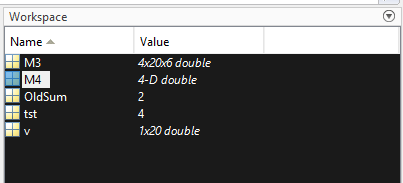
Side note, it’s impossible for us to think in 4D or higher. We just cannot do it, but we can do math in 4D and higher and sometimes it’s more computationally efficient to do so. You do need to be careful when doing that because it’s not intuitive and can lead to some issues. I try to work in 3D or lower, but on occasion 4D or higher will come into play for the work I do. It doesn’t happen often, but when it does I am extra cautions about checking the math and that I get the expected result from the operations I run. Normally when I need a 4D matrix it’s to take the mean across the 4th dimension and thankfully that isn’t hard to check since I can take the mean of the first entry across the fourth dimension and make sure that the value matches what I would expect to find. Below is the workspace showing a 3D matrix called M3 (4x20x6) and a 4D matrix called M4 (4x20x6x10). Notice that MATLAB only lists the 4D as 4-D

Now just because we cannot think in 4D doesn’t mean we can’t see what’s inside our 4D matrix. It just means we only get to see the 2D slices. Viewing a matrix in 3D makes no sense anyway because it would just look like a mess, so viewing the 2D slices makes it easy to see all the values. In MATLAB when we want to call the full length of a dimension we don’t need to specify the length we can just use the : symbol, so if I wanted to see the first layer of M3 I could call it like this M3(:, :, 1) where 1 is the layer I want and : , : in the first two entries tells MATLAB give me all the rows and columns. When we open the 4D matrix by clicking on it, a new window opens showing the entries using the same notation, but instead of 3 dimensions we see it written as M4(:, :, n, m) where n and m are any value up to the maximum value of our 4D matrix. We can scroll through our M4 matrix to see each layer and it will cycle through all the layers in the 1st “block” before moving to the second and so on.

This is the start of our 4-D matrix notice how the 4th dimension is 1, but the layer keeps changing. Once we get to 6, the highest value of our 3rd dimension, we will move onto the second block. Here’s the very end of our 4D matrix, remember the matrix is 4x20x6x10 so 4 rows, 20 columns, 6 layers, and 10 blocks.

There’s a few other types of variables we can introduce. There are also cell arrays. Cell arrays are useful because each entry is standalone, so they can be different types of data. We can store text into a cell array along with a matrix, a vector, or even a single value. The cell array doesn’t care because each entry is its own container where a matrix is is just a single container and everything going into it needs to be the same size and type. To make a cell array we simply use the {} instead of the () brackets we were using with a matrix. Cell arrays can be made by putting data in or you can just create an empty one and fill as you go. An empty cell array can be made using the following:

C{1,4} = [];

Which will create a 1 x 4 cell array. When you open the cell array all you’ll find is four entries with the [] symbols. They use the same convention as a matrix so it’s 1 row and 4 columns. Let’s toss in our 3D and 4D matrices into it just to show that it can be done.

C{1,1} = M3;

C{1,2} = M4;

Since each entry is standalone the cell array let’s me have both a 3D and 4D matrix inside. But let’s go wild and toss in some text since maybe we will forget that our arrays are 3D and 4D (we won’t but humor me). We can do that using the ‘ ‘ symbols. In-between those symbols we can add our text and MATLAB will treat it as a string. Like so

C{1,3} = ‘The first entry is a 3D matrix’

C{1,4} = ‘The second entry is a 4D matrix’

So now we have different variable types inside our cell array and all of them are different sizes, but MATLAB let’s us do this. This is great when I want to save some data (right click on the variable in the workspace for example and you can select save as, there is a way to do that via code, but we won’t cover that here). Using a cell array I can store several different datasets in one nice little package and put notes to remind me what each entry is from. This is great because after a few days of not working with the data I will forget what is what, seriously. It happens far too often to me so I label everything.

Lastly I can introduce a structure. If we think of a cell array as a folder for storing data, a structure is a bunch of folders. In neuroengineering, specifically EEG, we work with structures all the time. EEG is stored in structure format because we can store our data in a nice orderly way and name each “folder” so we don’t need to label things like we did with our cell array example. To make a structure we use a period (.) and name each folder. Say I want a variable with a list of colors. My structure variable may be named colors and inside I can add all sorts of different ways to create a color. Such as:

colors.red = ‘red’;

will create an entry in colors called red and inside that will be the text red. That’s not very useful since it’s just the same thing written twice, but say I want to store the hex code for green instead, that would look like this:

colors.green.hex = ’11BF0B’;

Inside colors is a “folder” called green, inside that folder is another folder called hex with the string 1BF0B. We can also add RGB inside and give each entry it’s own “folder” or as MATLAB calls them fields such that:

colors.green.RGB.R = 17;
colors.green.RGB.G = 191;
colors.green.RGB.B = 11;

Double clicking on the variable colors will open the window below

Now I’ve cheated and opened the green folder, you can type this out in the command line by calling colors.green and it will print the values shown below (not exactly displayed as you see below) or you can open the “folder” by double clicking on it like I did in the capture below.

You’ll notice we can go even further and open RGB, to do that in the command line it’s just colors.green.RGB, or double clicking will display the screen below.

For completeness if you type it in the command line, MATLAB will return the values like this:

since I did not specify a variable to store this information in MATLAB will automatically designate it as the variable ans and anytime you type in a command without giving the variable a name ans will update with the latest values MATLAB returns. It’s a weird quark of MATLAB, but it works in your benefit on occasion if you need the value later. If you plan on using the value for anything other than practice, you should always give the variable a real name and don’t rely on ans because MATLAB will inevitably change the value of ans. If I entered 2+2 in the command line MATLAB will return ans = 4, if I say ans+2 MATLAB will give me ans = 6, it won’t give me a new variable for ans, it will just replace it. In short, don’t do it for code you will use on a regular basis, you don’t want that headache.

I think we’ll stop there for today since this is getting excessively long for a single post. Remember each class was two hours long roughly so transcribing everything I taught in the class is hard. For that reason I’m attaching the example code which is full of useful hints, tips, and suggestions. Basically I cover the things I’ve learned the hard way because I’ve made the same mistakes I’m warning you about. You don’t have to be like me!!

Keep in mind you don’t need MATLAB to view it, any text editor (word, notepad, etc. will open it, it just won’t be nicely colored. Since WordPress hates the .m file type apparently, I’ve put it inside a zip file since that was the only way to get it to upload. It’s safe, you can scan it if you don’t trust me (I don’t blame you, you don’t know me), but it’s here if you want some examples of the stuff above for your own personal use here it is.

For the record, I’m cool with you sharing the code with people, it’s why I wrote it. However, I put a lot of time and effort into this class so I would apricate you linking back to my blog if you do share it. Credit isn’t that hard to give, so please give it and I’ll be happy with you sharing. That’s what knowledge is for after all.