Day 19: The Central Limit theorem

Well here we are again, if you recall from our last post, we talked Bonferroni Correction. You may also recall that when the post concluded, there was no real topic for today. Well after some ruminating, before we jump into more statistics, we should talk about the central limit theorem. So let’s do a quick dive into what that is and why you should know it!*

We glossed over a few important things that we need to cover and this is one of them. Waaaay back in this post, I said that when we use parametric statistical analysis we make several assumptions about the data we have. I’ll go over parametric statistics and nonparametric statistics explicitly in other posts (note to self…), but one of the assumptions was that our data was normally distributed.

We sort of glossed over the idea that we just make this assumption and really who are we to assume anything about the data we collected? Right…? Well it turns out that people far smarter than I have come up with some guidelines for this sort of thing that allow us to make this assumption and it turns out that it is a fairly robust assumption to make. Enter the central limit theorem.

The central limit theorem states (somewhat confusingly at least to me) that any set of variantes with a distribution having a finite mean and variance tends to be the normal distribution.

Let’s break that down if you don’t understand what that means exactly (don’t worry, it is confusing). What it means is that as our sample size gets larger, the sample means approach a normal distribution, no matter what the shape of the population distribution.

Now, when we say sample means, we don’t mean the population mean, that is different. Our population is what we call all our collected data. However, suppose we look at a subset of our population and took the mean of that subset, that is the mean of our sample which is not equal to the mean of our population. Let’s use an example to clarify all of this.

Let’s say we have 1000 cats (let’s assume an animal foster care situation and not crazy cat person situation) and we are interested in the average size of those cats. So we a measurement of each cat and find the mean of all 1000 cats, that would be the population mean. If we plot that data in a bar plot it may look something like this:

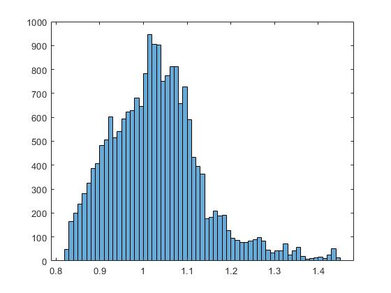
Example cat distribution

That doesn’t look normally distributed! But that isn’t what the theorem says. It says if we take the mean of samples of our population it will be normally distributed.

Back to our cat example!

Instead of looking at all the cats, say we measure 5 and take the mean of that subset. Next, say we repeat this process 100 times, that would be 500 cats, only half of our population, but what you would find is that if we plot that data in a bar plot we should find that it is normally distributed (OR, at least approaching normally distributed, because we have a finite set and remember the theorem says that as our collection of means gets larger, we will see our data become more normally distributed. In the end we would end up with something like this:

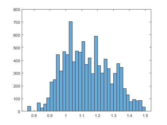
Distribution of the means of our subgroups

In this case, our data still doesn’t look perfect, but you can see that it is in fact fairly normally distributed. So let’s recap really quick in a list so we can make sure we get this:

• We have a population of 1000 cats
• We take groups of 5 cats and determine the mean of that group
• We repeat this as many times as we want (in this example we did this 100 times)
• The histogram of this data will be normally distributed.
• The larger the means of our subgroups (say had instead 10,000 cats and we took mean of cats cats in groups of 5 and repeated this 1000 times), the more normally distributed the data will look.

This has interesting implications because while the values we collect from a population might not be normally distributed, the means of a set of subgroups in the population WILL be normally distributed. We can look at some examples where normally distributed data comes in handy, but if we remember that we already discussed the parametric statistics requirement that our data be normally distributed, we already see why having normally distributed data is important. Don’t worry though, we will go over other reasons later. Not bad for not having a topic for today, right?

Until next time, don’t stop learning!

*As usual, I make no claim to the accuracy of this information, some of it might be wrong. I’m learning, which is why I’m writing these posts and if you’re reading this then I am assuming you are trying to learn too. My plea to yu is this, if you see something that is not correct, or if you want to expand on something, do it. Let’s learn together!!