Day 40: The Normal Approximation (Poisson)

Poisson’s return!

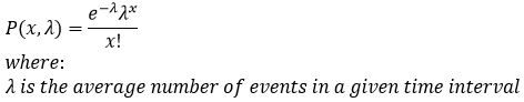
If you haven’t already, you should read the Poisson pdf post. In anycase, if you’ve been following along we usually do a recap of the related bits before we get into something new, this is no different so let’s talk Poisson. This is the Poisson pdf mathematically:

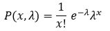
We also rewrote it so it looked slightly similar to something else we’ve seen (the exponential pdf), where the rewritten Poisson pdf looks like this:

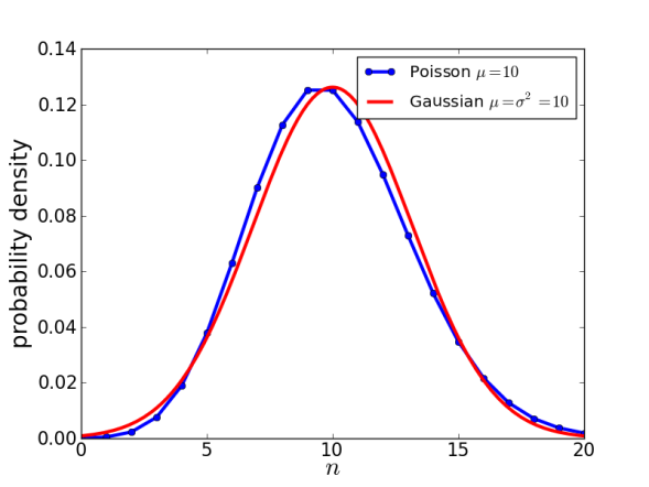
We also saw that as our λ value increased, the resulting pdf became more and more gaussian looking. If you look at the picture at the top of the post, you can see that as μ gets larger (in that case μ = 10) we get a distribution very close to the gaussian. If you are confused, don’t worry, μ is just the mean of the Poisson pdf, so really μ = λ and this is a variable swap that you will see fairly frequently so you may want to get used to seeing it written both ways.

Like we mentioned last time, the binomial distribution is discrete, we hate this in math because we are lazy and want to be able to integrate the thing, which we cannot do unless it is continuous, so we find ways to approximate it that will give us a continuous function that is close to the discrete version we are dealing with. Now we’ve already talked about what the binomial distribution looks like, you can read about that in the last post, so we won’t get into it. However you should probably be familiar with the notation as we go on. I’ll do my best to explain it, but that post does a fairly good job (in my opinion) of breaking it down.

That said, let’s look at the binomial approximation using Poisson this time. That looks like this guy:

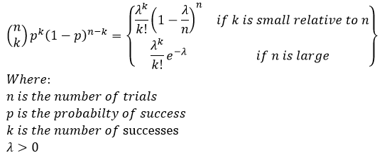
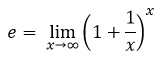
You may be wondering where the e came from in the case where n is large, well I was confused by this at first too, but have no fear, this should help. You may remember that e is a special number, e = 2.718… but that number isn’t just a random number someone picked. That number is found by this equation:

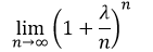
If you look at our first version of the binomial approximation (where k is small relative to n) you’ll see a value that looks strangely close to this definition, this guy which we will call (1) for the moment:

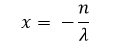
It’s not exactly the form, but we can get it there if we do a quick substitution:

When we substitute this back into (1) and we get this:

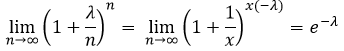
So the term just simplifies to what we see in the second version of the equation (if n is large), this is because we need n to be really big to make the substitution. Of course, this in itself is an approximation (because again we want to be lazy!) and we will never see a real life case where n is ∞, so how big does our n need to be to make this approximation so that it is valid? Well that is an excellent question with no real clear answer. This is an approximation so it depends on how accurate you really want to be. Basically we want n to be large and np to be small, where λ = np. We typically want to find a λ > 10, (np > 10) to use this approximation. This is why we can’t really give a direct answer, because it depends on the values of n and p to determine if this approximation holds in your case.

Additionally, if you look at the example plot at the top if the post you’ll see that our np = λ = μ = 10. Yeah, I know that might be confusing, but they are just variables meaning our mean value of the data is 10 and the change in variable is just a change, not some hidden math, they are equal.

Okay, well that introduces the Poisson approximation. Why would we use this over the gaussian approximation? Well again, we want to be lazy, no that isn’t a bad thing, we don’t want to have to do a lot of work and this equation is arguably easier to solve than the gaussian approximation. However, there is the limitation where we want to see λ > 10 before this holds, so we need both for a complete approximation (in cases where λ < 10.

The lingering question is probably how does this all relate to everything we covered? Well, next post we can get into it and talk about how these things relate. Then moving forward we can get into some of the other topics so I can stop playing catch up with the class I am in and we can get into the current things we are covering!

Until next time, don’t stop learning!

*My dear readers, please remember that I make no claim to the accuracy of this information; some of it might be wrong. I’m learning, which is why I’m writing these posts and if you’re reading this then I am assuming you are trying to learn too. My plea to you is this, if you see something that is not correct, or if you want to expand on something, do it. Let’s learn together!!