Day 39: The Normal Approximation (De Moivre-Laplace)

The binomial distribution, don’t worry we’ll get into it.

Say we are interested in flipping a coin. Now let’s say we want to do that a few hundred times, sort of like our coin flipping example! If we wanted to determine the pdf based on the total outcomes of the experiment we would see that we have a plot that looks very gaussian… but it isn’t.

This is because a gaussian pdf is continuous, where a heads or tails experiment is very much a discrete experiment. We call this distribution the binomial distribution and the math for it looks like this:

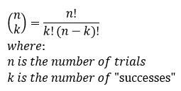
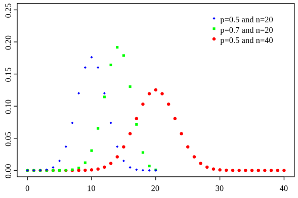
You would read the bit on the left side of the equals sign as n choose k. This just means given n trials how many “successes” would we have. We define successes as outcome we want, in our coin flipping experiment we could define success as either a heads or a tails and we could ask what are the odds we get 10 heads after 100 trials, which would be n = 100 and k = 10, or we could ask what is the probability that we would get 10 heads after 10 trials (n = 10 and k = 10). At first, this doesn’t look familiar at all and you may be thinking that I’ve gone crazy trying to relate this to the gaussian, however if we plot the pdf we see it looks like this:

Notice that instead of a line we have discrete points, that is because unlike the gaussian, this is a discrete distribution so we typically represent these using points. This can get a little confusing as the number of points increases to infinity, but you can see what we are leading up to if you think about that situation.

This was the realization that de Moivre and Laplace came to, as we increase the number of trials we can use the gaussian distribution (remember, it is also called the normal distribution, but it is the same thing, so don’t get confused) to approximate the binomial distribution. If you remember our plinko game animation, you will know we’ve already seen an example of this!

Notice that in this case, each ball represents a trial, so that ends up being a lot of trials! That is good however, because (as you can see) it works out to be a really accurate representation of what amounts to a probabilistic process. So what does this approximation look like? Well the equation looks like this:

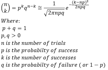
If you notice, this approximation becomes more and more accurate as n increases. This should make sense if we think about it in terms of what we are trying to represent. We will not go through the proof of this theorem (nor do I think you want to), but you can and it is readily available online if you want to see how we go from one to the other.

Let’s talk about the why, why use this, what are we even doing and why does it look so much more difficult?! Well, if you remember back at the start of these posts we discussed using integration and we said that being able to integrate makes the math easier. This is still very true, so being able to use a continuous approximation of the discrete pdf gives us the ability to differentiate and solve for the CDF! In fact, this is still used to this day, even with all of our awesome computing power. Granted, you can still use the binomial pdf, but it is less computationally intensive to use the approximation, which is sometimes important when working with really large sets (very large n values), which to be fair makes the approximation more accurate anyway.

Okay, so what does this all have to do with what we’ve been covering? Well we can talk about the other way we can approximate the binomial distribution tomorrow. For now though, I think we’ve got to a good place. Stick around though, we’re going to start rapidly connecting the dots here in just a few posts.

Until next time, don’t stop learning!

*My dear readers, please remember that I make no claim to the accuracy of this information; some of it might be wrong. I’m learning, which is why I’m writing these posts and if you’re reading this then I am assuming you are trying to learn too. My plea to you is this, if you see something that is not correct, or if you want to expand on something, do it. Let’s learn together!!