Day 46: Functions of One Random Variable Example Part 2

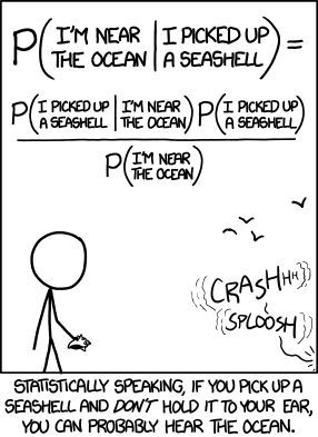
Another Joke by xkcd

As promised today we are going to look at another example of how to solve functions with one random variable. If you haven’t you may want to start with our first post on the subject here.  For those of you who are caught up, let’s get started.*

So last example we looked at we used the method of distribution functions to solve for a Y(X) = g(X) where X was a random variable with a distribution function attached to it. Today we are going to use moment generating functions to solve for a random variable so we can see what that would look like.

Let’s say that X is normally distributed where X ~ N(0,1). Now say that

This gives us a function of a random variable (Y) that we can now solve using moment generating functions (MGF) to solve this. First let’s look at our MGF and then plug in our equation, remember this is a normal distribution so we already know what X looks like and how to solve for it. So if you recall our MGF looks like this

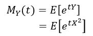
All we did here was take our MGF and plug in our Y value since we said that Y = X^2. Now we are going to solve by integrating the entire space, so from -∞ to +∞ (because that is where our normal function “lives.” Now I’ll go through a couple of steps and we can talk about the result at the end.

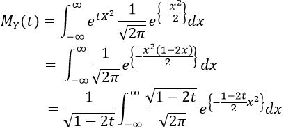
This might be a bit confusing, so let’s look at what we did first and I’m sure we can make sense of this. You’ll recognize the gaussian (normal) equation that we put in, the mean is zero so we don’t have the μ term in the exponential. So now we have two e terms raised to the power of something and in the second step we combine the like terms. In the last step we do a (somewhat) change of variables to make this easier to solve (you’ll see in a minute). This let’s us pull out the constant (since we are integrating for x, not t) and it looks like we made the equation more complicated, but really all we did was rewrite it so we now have a normal distribution where

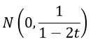
However, we are taking integral of the normal from -∞ to +∞ so we know this sums to 1 because it’s the full space, meaning all that is left is the stuff outside the integral. This means that our equation becomes

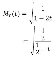
(where we divide out the 2 in the 2t)

This is the MGF of a gamma function where Γ(1/2, 1/2), which means we now know the distribution of our Y! Pretty neat right? I think we will go over one more example tomorrow and then look at the inevitable one function of two random variables bit. After we do that, then we should be able to generalize and solve for one function of n random variables. There are some techniques that will let us make this generalization, so we’re going to talk about the jacobian… eventually. In any case, we’ve got a plan for the next several posts.

Until next time, don’t stop learning!

*My dear readers, please remember that I make no claim to the accuracy of this information; some of it might be wrong. I’m learning, which is why I’m writing these posts and if you’re reading this then I am assuming you are trying to learn too. My plea to you is this, if you see something that is not correct, or if you want to expand on something, do it. Let’s learn together!!