Day 246: The Kalman filter

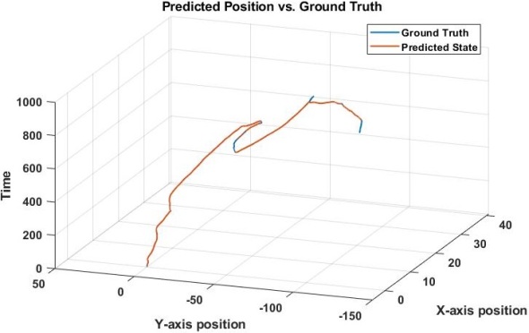
This is just one application for the Kalman filter, I estimated a two dimensional position using a random walk model. We have 3-dimensions here even though it is a 2 dimensional problem, the third dimension is time. This way we can see the path over the course of the recorded time. Notice there are no units, becuase in this case we were working with synthetic data so the units were meaningless and I did not include them.

Since we’ve been talking a lot about it, I thought it might be a good idea to formally introduce the Kalman filter. This will be a semi-high level introduction (like my knowing your spinal cord series), but at the end of it you should have a relatively good feel for what a Kalman filter is.

First, let’s get this out of the way, there are several different types of Kalman filter out there. They all have different use cases and reasons for why a certain Kalman solution may be better than another, but at the end of the day they are all basically made of the same thing. There are two steps to a Kalman filter, the prediction step, and the update step. Let’s go over each before we look at the formula for the kalman filter itself.

The prediction step is simply defined as a estimate of the current state based on the previous measurement. Now I said state, don’t be worried, a state is literally what it sounds like, a state of being. I like to use a lightswitch as an example, it is a binary process so it only has two states an on state and an off state.

Let’s run with that for our example as I talk you through the Kalman filter. Say we want to know the state of the lightswitch without looking at it. Let’s further say we are measuring ambient light conditions, that seems like a good way to tell if the light is on or off. However we have the sun to contend with so we need a model, I’ll skip over how we build that model for the sake of clarity in this case, but there is also another problem. Any measurement we take will have some noise associated with it, this could be sensor error, reflections, people walking by the sensor, whatever. It’s all noise! So we only have a noisy measurement to estimate our state!

So we take our measurement and feed it into the first equation, our prediction step, the equation for which is shown above. This looks very complex, but it isn’t I promise. A is a n by n square matrix and is called our state transition matrix. This is something that we need to calculate, so I’m going to gloss over the how here becuase that is a whole other can of worms. x is our measurement and Q is our noise associated with the measurement. So we’ve made our measurement, now we predict the next value we should get.

We now have our estimated value, so we can take a measurement again and see if it is correct. This is where we get into the update step. The update step takes our estimated measurement, compares it to our actual measurement and adjusts something called the kalman gain (literally a gain, so a multiplier that raises or lowers our prediction) and the process starts all over again. The fancy math behind our update step is shown below.

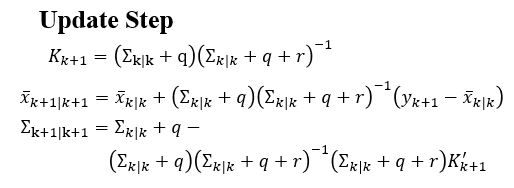
K is our kalman gain and the tiny k+1 just means our kalman gain for our next prediction (hence the +1). This step helps adjust our kalman filter so we have an accurate prediction, but to have an accurate prediction we need to have a good model. So much work, right? This is an iterative process so after every prediction, we have an update and in the end, we get a very accurate prediction when we have a very accurate model and a not so good prediction when our model is bad.

In this case our model consists of an A matrix (explained above) and the noise for both our measurement is that Q, we also have this  ∑ (epsilon) term and that is our uncertainty around our measurement, I like to think of it as our confidence in our measurement. So we have four(ish) depending on the model things we need to solve for to get a good model of our system. To do this, we can use expectation maximization, which is something we will go over some other time (probably tomorrow).