Day 1: Power Spectral Density (pwelch)

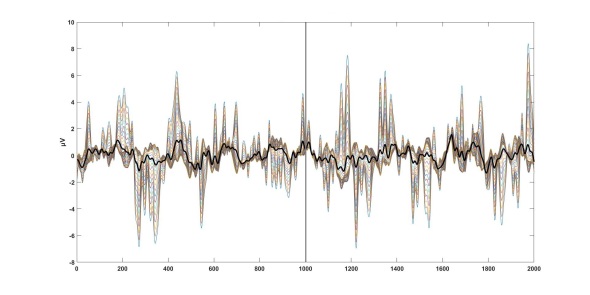
Some EEG data that I’ve aligned, processed, and made look nice and pretty.

Signal processing, it’s complex, there are a million ways to go about processing a signal, and like life, there is no best way to go about doing it. Trust me, it is as frustrating as it sounds. Today’s scratch pad note is on power spectral density or PSD for short. So let’s dive in.*

So you’ve collected some data, good! Well one of the first things we can do with that data is look at the power spectral density. For this post (and most future posts I’m sure) I will be using MATLAB, but with some work you can translate it to just about any other programing language. Like I mentioned earlier, there are a bunch of ways we can do this, but the two we will be talking about today are Welch’s power spectral density estimate (MATLAB command is pwelch) and Thomson’s multitaper method (MATLAB command is pmtm). Both methods rely on the same basic principle, the Fourier transform.

The magic of the Fourier transform is that we go from working in the time domain to the frequency domain where a whole lot of difficult calculations become much simpler to solve. This is done by approximating the signals using sine and cosine. This transformation means we can look at what frequencies make up the signal (among a lot of other useful stuff) and while it is just an approximation, we can get really close, as in close enough to be a valuable tool when doing signal analysis.

So in the spirit of being somewhat to the point, let’s talk about the MATLAB functions specifically and what the parameters mean. I’ll go over pmtm tomorrow, but for today, let’s talk about the pwelch command:

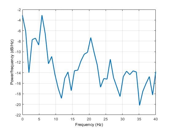
Example of the pwelch output (the data was noisy, as you can tell by how jagged it is.

[pxx,f] = pwelch(x,window,noverlap,f,fs)

There are quite a few inputs, some easier to figure out than others, in this example:

Inputs:

• x is your signal, that should be straight forward enough.
• window allows you to specify window size
  • A larger window will give you better frequency resolution, but with a cost, it increases noise (because you are averaging across fewer windows).
  • A smaller window will give you more total windows so the noise (assuming it is really random) will be reduced.
• noverlap, this is the overlap size (n) for the windows (hence n-overlap, not no overlap, which is how I read it at first… oops)
  • The question is how can we use large windows and still have enough windows to make a smooth plot, overlap is the solution. With computing power where it is now, you can crank up the overlap to window – 1, it is a diminishing returns thing and once you have ~70% or so of overlap you’ll see minimal improvement, but again if you’re doing this processing on a computer, you shouldn’t have an issue. If you are doing it on a microcontroller or something that doesn’t have power behind it, then you may want to play with it.
• f, this input (not to be confused with the f output) is the frequency(ies) of interest (ie the ones you specify with this, I’ve never used it, but yay for completeness!
• fs, this is the sampling rate of your input signal (x), you do know your sample rate… right? This translates the output to Hz instead of the normalized frequency that will be outputted (x π rad/sample).

Outputs

• pxx, this is what we are interested in, the transformed signal. When we plot, the y-axis will be in dB/Hz or if you didn’t specify the sample rate (fs) then your output will bein dB/(rad/sample).
• f, this is is your frequency vector, basically this is your x-axis so if we oversimplify everything your outputs are your y-axis and x-axis.
  • Note: if you did not specify your fs, then MATLAB documentation has the variable f as w (the normalized frequency vector) so while they aren’t interchangeable when we talk about them, they are related.

You can also specify a bunch of other things, such as confidence interval, range, nfft (which I will cover at a later time), and a few other things.

So not a deep dive, but still a fairly long intro into pwelch. We did not cover how this differs from pmtm, the window shape (because yes you can shape the window and this has important ramifications for your output), we haven’t talked spectral leakage (no one likes leakage), and we haven’t covered a bunch of other stuff. On the other hand, we have 364 days left so I think it will get covered soon(ish).

It’s day one of 365 days of academia. So far so good, look at me sticking to goals! I doubt they will all be this long, but hey a strong start.

• I should note that I make no claim to the accuracy of any of this, so you may want to verify, but hey if you find something, say something. I’m learning, you’re learning, let’s learn together.