Day 4: Spectral leakage… embarrassing

Look at that leakage!

Leakage, it’s never a good thing. For today’s post we’re going to cover a very important topic. Spectral leakage, it’s a big reason why spectral density estimation is well, an estimation. The other reason it is an estimation is because the fourier transform is an approximation of the original signal, but the Fourier transform is a whole other post on its own. So let’s talk leakage!*

In our last post, we talked about Welch’s method and Thomson’s method, both use windows to estimate the power spectral density (PSD) of a signal. Welch came up with the idea of overlapping the windows and Thomson decided he could take multiple measurements from the same point in time of the signal by changing the taper of the window and averaging them for a more accurate estimation of the component frequencies (hence his method being called the multitaper method). While they are very similar they are also very different! We also saw that the spectral density of the same signal could look quite different depending on which method you use (our example PSD comparisons from yesterday is shown again below). Part of the problem comes from the windows and how everything is averaged.

Power spectral density calculated using PMTM

The same signal, but this time the power spectral density is calculated using pwelch

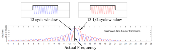
If we look at the spectral density estimate above, we see that our window selection biased our output (the blue output is centered around 13 Hz while the red output is shifted by +0.5 Hz), but why? Well the answer is complex, but the main issue is that our window is finite. This creates leakage when we have a signal being analized that isn’t perfectly periodic in the length of the window. Furthermore, because we use a sliding window, we are guaranteed that at least part of the window will not be perfectly periodic (ie selecting the full period of the frequency in the signal). This is why when our window is 13 1/2 periods long, even if our signal extends the full length of the window, we get a shift in the estimate (we also get that periodic attenuating wave shape for the output).

This output is also a good representation of what we mean when we talk about the main lobe and side lobes. We can get into that next time, however the main point is that the shape of the window we use (it isn’t just a rectangular window like our example is) will have an effect on the main lobe and side lobes. The wider the main lobe the smoother the signal will look, but the less resolution we will get (because it is wider, more signal frequencies fit into it).

If we look at the image above, the blue transform is centered around 13 Hz. Easy enough, but you also see that it isn’t a peak, it gently curves, eventually reaching zero dB at 12 and 14 Hz. This is our main lobe which is dictated by our window shape (again a rectangular window). While this makes it easy for us with our prior knowledge that the signal is a pure 13 Hz frequency, it would be much more difficult to do the same thing if our signal was more complex and made up of more than one frequency.  More importantly if we didn’t know what our signal was composed of, it would be easy to look at that and think our signal may be made up of additional frequencies close to 13 Hz and not only 13 Hz. This is where prior knowledge of our signal helps, so we can select a window size and shape that best fits our sample signal.

This only goes so far of course, but if we know that our signal is between 10-40 Hz, based on our sample rate (Fs) we can adjust our window size smaller than we would if we were interested in frequencies between 1-30Hz. Because a 1 Hz signal period is much longer than a 10 Hz signal period so if we want to capture that in our analysis we need to have a much larger window than if we were only interested in the 10 Hz.

Let’s tackle some more of is next time, but for now I think this is a good spot to stop. We’re starting to get into some really interesting concepts, so I hope this is all making sense. Next time I think I’ll talk window shape and its effect on our main and side lobes. I skipped over the Fourier transform so at some point I should go back and over that too since it is the basis of everything we are talking about (more of a note for myself really since I try to read over these on a regular basis).

So until next time, don’t stop learning!

*Friendly reminder, I make no claim to the accuracy of this, I’m learning and if you’re reading this then you are probably learning too. If you see something that is not correct, or if you want to expand on something, please do. Let’s learn together!!