Day 5: Whose window function is it anyway?

This is not how we use a window function on the computer…

One day someone looked at the windowed fourier transform and said, “Don’t be such a square!” and thus window functions were invented. If you believe that, then I have an island for sale, real cheap. But seriously, let’s do a dive into what a window function is and why the heck there are so many of them, because there ARE a LOT! So let’s get started!*

This is sort of what we’ve been building up to, what exactly a window function is and why we need it. Last post we covered spectral leakage! In short, spectral leakage is the error of the spectral estimation due to the finite length of the window. In other words spectral leakage occurs because the frequency doesn’t always fit nicely inside the window so the estimation gets skewed. We can minimize, but we cannot get rid of spectral leakage. This is why Welch’s method uses overlapping windows and why Thomson’s method uses multiple tapered windows, both methods try to overcome the problem with windows (insert microsoft joke here).

Now, every window function, from the basic square window to fancy shaped windows have what is called a main lobe. The main lobe is the center of the window, it is where the weighted average is at it’s highest and it has a particular “shape” to it. This also gives rise to side lobes, these are caused in part by the effects of using finite window to analyse a finite signal. The main lobe and the side lobes all impact the averaging so when you’re looking at the window shape, you are also looking at how the signal is weighted, the higher the lobe, the more weight is given to it.

Now that we’ve gone over what the shape of the window means and what it does, let’s look at different window functions to see what effect it has on the signal of interest. First let’s look at what the square window looks like in terms of the Fourier transform.

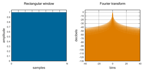
Square window (left) and the output from the Fourier transform (right)

The image on the right shows what the window looks like to the Fourier transform. Remember, the peak at the center is our resolution of the frequency of interest, the wider the main lobe, the lower the resolution, but the smoother the output will look. The higher the peak, the more weight it has in the average. If we look again, the side lobes drop off at a very gradual, meaning that other non-target frequencies get weighted into the average as well. But what if we change the shape? Let’s look at a different shaped window, here is a still fairly simple triangle window.

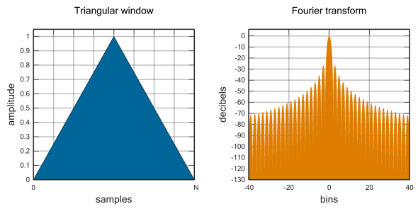
Triangle window (left) and the Fourier transform of that window (right)

The main lobe (seen in the right image at bin 0) is wider than the main lobe above. This is the trade off we deal with when we select a window shape, notice that even though the main lobe is wider, the side lobes drop off faster and more drastically than the square window. This is good in that the side lobes don’t contribute as much to the output, but we still lose frequency resolution due to the wider main lobe. Okay, well a square window and a triangle window have different trade offs, but what if we use something in between the two? Let’s look at the Welch window (I’ll let you guess who came up with it).

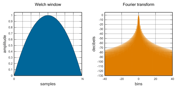
Welch’s window (left) and the Fourier transform of the window (right)

Now we’re getting somewhere. If you look at the main lobe, it looks smaller than the triangle window yet still larger than the square window. Additionally, the side lobes drop off faster than the triangle window and square windows. This increases our frequency resolution and further eliminates the skewing caused by the side lobes of the window. So now you may be thinking that a more complexly shaped window may give you the best of both worlds, high frequency resolution AND little contribution from the side lobes, well let’s take a look at something called a flat top window.

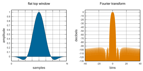
Flat top window function (left) and the Fourier transform of the window (right)

Wait, what just happened? You may be wondering what’s going on, well here the function has a partially negative weight so we can eliminate some of the contribution from the side lobes, if we look at the transform, we see it does just that and very well. However, the main lobe is the widest we’ve seen yet and this perfectly highlights our dilemma. If we want to eliminate side lobe contribution we will lose main lobe resolution. Unfortunately this is just the nature of the transformation, so we must come to deal with it in other ways.

The way we do this is a whole lot of different window shapes. No really, there are a bunch. In fact, all of these images are directly from the wikipedia page on window functions. You can see there are far more than I could cover and there are others that the page doesn’t mention. The thing is, using our prior knowledge of the signal we can select a window that works best for our analysis. So if the images are from wikipedia, why am I writing all of this instead of just referencing the wikipedia? Well first to learn, second they go into detailed mathematical explanations on how the window is defined. Let’s face it the wikipedia page is very, very dry and some of us just need an overview or an understanding of the key concepts. I sincerely hope that I’ve accomplished that here.

With that, I think my work here is done for the day. Next time we can talk about the lynchpin of this whole thing, the Fourier transform! Or maybe we will cover something else. I haven’t decided yet, but it will be good. So until next time, don’t stop learning!

*Just remember, I make no claim to the accuracy of this, I’m learning, which is why I’m doing this. If you’re reading this then you are probably trying to learn too. If you see something that is not correct, or if you want to expand on something, please do. Let’s learn together!!