Day 6: The fast and the Fourier

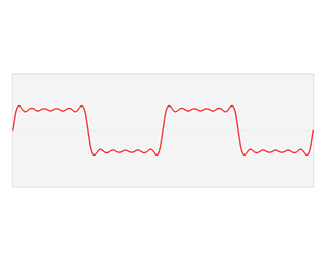
A good example of how the Fourier transform can approximate signals. The red signal is our input signal and the blue shows how the output of the Fourier transform.

Okay, if you’ve been keeping up with these posts, we know about Welch’s method, Thomson’s method, the things that make them different, and the things that make them similar. The thing that both of these transforms rely on is the Fourier transform. What is the Fourier transform? Well, something I probably should have covered first, but whatever this is my blog we do it in whatever order we feel like, so let’s dive in!*

What a ride, we’re almost a week through 365 Days of Academia (365DoA) and I feel like we’ve already covered so much. One thing that has been bugging me about all of this is that I missed going over what the Fourier transform is and it is the whole reason these methods even exist. 

The Fourier transform — according to wikipedia — “decomposes a function of time into its constituent frequencies.” You may remember that I mentioned last post wiki was very dry… right? But what exactly does decomposing a function mean and more importantly why do we care if we decompose a function?

Way, way back (1822) Fourier showed that any signal could be approximated as an infinite sum of harmonics. That’s just a fancy way of saying that if we keep adding sine and cosine functions together at different frequencies and amplitudes we can recreate very complex signals. This is good because if we have a signal that looks like a jumble of oscillations, finding a relatively simple equation that creates that signal is all but impossible.

This is why we say we can go from the time domain to the frequency domain, because we are no longer looking at our input signal in terms of time, but in terms of frequencies (and amplitudes). Also remember, sine and cosine by their nature are infinite, this has some implications we can discuss later. More importantly is what we can do when we take a complex looking signal (especially one we don’t know the equation for) and apply the Fourier transform. Going to the frequency domain makes math much, much simpler.

When we go from the time domain to the frequency domain, if we are typically dealing with a set of linear differential equations (hard!!) they become algebraic equations (simpler). For those unfamiliar with differential equations, linear differential equations they can be (literally) impossible to solve.  The bad thing is that a LOT of natural processes can be represented using linear differential equations, which is why we use them so much. That’s the power of the Fourier transform and why it comes up so much, because algebraic equations are far less computationally intensive.

To be complete I need to mention that there are a few different ways we can go from the time domain to the frequency domain, but one of the more widely used methods is the Fourier transform. Why? Well one reason is there are a lot of equations that are already mapped for the transform, so if you can identify the equation that describes the input signal (this is done a LOT in controls, where I first really learned how to use the Fourier transform), you can easily convert to the frequency domain. This can involve rewriting the input function in terms that meet the format of already mapped equations, but the point is they exist and make it easy to go from one domain to the other and back again (using the inverse Fourier transform). You can also do this (somewhat) brute force if for example you’ve recorded some signal and have no clue what the function could be and in fact we’ve covered two different MATLAB functions that do just this!

This actually has very practical applications in data compression, signal processing (which is where I use it these days), and all sorts of different science applications. There are also some interesting limitations and we’ve already hinted at this.

When we use the Fourier transform to approximate a signal in the frequency domain we are making a very large assumption. We are using the infinite length sine and cosine functions to represent finite signals. This is where other transformations and approximations come in, one of these is called the wavelet transform and specifically addresses this issue. However, I think we’ve done a pretty good job of introducing the Fourier transform so we can cover wavelets some other time!

Remember, don’t stop learning!

*As usual it is important to remember that I make no claim to the accuracy of this. I’m learning, which is why I’m doing this. If you’re reading this then you are probably trying to learn too. If you see something that is not correct, or if you want to expand on something, please do it. Let’s learn together!!