Day 7: Small waves, or wavelets!

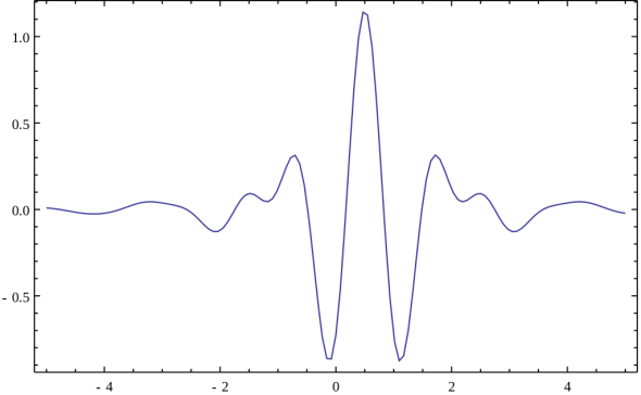
This is the Meyer wave, a representation of a so-called mother wavelet function to use for the wavelet transform. Notice that it is finite!

Waves! We’re officially one week through 365 Days of Academia! Woo! 1 week down, 51(.142…) weeks left! Let’s wrap up this weeks theme (there wasn’t originally a theme, but it kind of ended up that way) by talking about other ways we can get to the frequency domain. Specifically, let’s stop the wave puns and let’s talk wavelets!*

Last post (Day 6) we broke open a whole can of worms named the Fourier transform. I touched on why it was important, a little about what we could do with it, and one very important assumption. If you forgot, don’t feel like reading it, or just want to hear it again the assumption is this, we are taking a finite input signal and transforming it using the sine and cosine functions. In other words, we are taking a finite input and describing it using infinite terms.

Enter wavelets…

The Fourier transform can be thought of as being localized in frequency only, this is because they are infinite waves, this is actually a special case of the continuous wavelet transform. In this case the mother wavelet is going to be your sine or cosine functions.

Wavelets on the other hand are finite wave functions, simple right? In this way wavelets (in the general sense) are localized in both time and frequency. If you remember the window function discussion, we hit a resolution issue which was limiting our output, we either saw a high frequency resolution (the width of the main lobe) or a lower contribution by the side lobes, but no matter what window function we selected we ran into this trade off.

Wavelets don’t have this issue, we can stretch the mother wavelet function in both time and amplitude to better approximate the input function. Additionally, we are not limited to our mother wavelet shape, there are several wavelet functions with their own shapes that we can select from. What’s even crazier, the discrete wavelet transform is less computationally complex than the fast Fourier transform.

Interestingly this has nothing to do with the transform itself (it is still computationally intensive), instead it is because we can logarithmically divide the frequency instead of being forced to have equally spaced frequency divisions like we deal with when using the fast Fourier transform (which is the name of the algorithm we use to calculate the Fourier transform, so don’t worry when we say fast Fourier transform, at the core it is the same thing essentially).

So that is your crash course in wavelets! We can do a dive into what exactly a mother wavelet is, but essentially it’s just the shape of the wave you are using to calculate the wavelet transform. I’m not sure what I plan to cover next, but I’ll think of something.

As usual, don’t stop learning!

*Everything here is 100% correct, not really! In fact, I make no claim to the accuracy of this information, some of it could be wrong. I’m learning, which is why I’m doing this. If you’re reading this then you are probably trying to learn too. If you see something that is not correct, or if you want to expand on something, please do it. Let’s learn together!!