Day 8: The Spectrogram Function

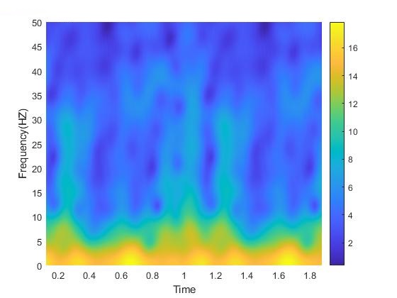
Example spectrogram from some data I had recently processed

To (somewhat) continue with our signal processing theme that we have going on at the moment, over the next few days, let’s look at something called the spectrogram. It’s three dimensions of fun!*

Since we already covered a couple topics in a particular order, let’s go ahead and do that this time. Using our previous posting format it would be prudent to go over the MATLAB command to create a spectrogram and then over the next couple of days we can dig into what it is exactly and what it does. Frankly, this might be the topic for the rest of the week. So let’s dive in with the command:

[s, f, t, power] = spectrogram(Data,window,noverlap,nfft,Fs)

Inputs

• Data – signal you want to run the spectrogram on, easy enough!
• window – if you’ve been keeping up with our posts, you know that the fourier transform is calculated using overlapping windows, this is your window length. The bigger the window, the better frequency resolution. IE if you have a 1000 sample/second rate, then if your window is 500 you can only resolve signals that are greater than 2 Hz because your window isn’t long enough to capture the full 1 Hz waveform.
• noverlap – don’t read this as no overlap (one too many o’s), its n-overlap as in the number of samples to overlap your windows. Statistically setting this above ~70% won’t give you much improvement to your analysis, but if you have the computing power to do it, you can do window-1 (or maximum overlap) and it won’t hurt, but it may not help… much.
• nfft – this is a little more complex in the sense that the documentation doesn’t do much to explain it and there is a bunch of conflicting information on what to select. This is how many FFT (fast Fourier transform) points are calculated per window. A higher nfft will give you a higher frequency resolution. The defalt is either 256 or floor(log2(N)), where N is your signal length and floor just rounds the output down to the next integer. You can play with this value and see what your output looks like, it can get choppy looking if your value is too low.
• Fs – your sampling frequency. You should know this because it impacts the calculations.

Outputs

• s -the short-time Fourier transform of the signal, basically what you are interested in, or you can do what I do and use the power option (keep reading and I’ll explain what I mean).
• f – a vector of frequencies. If you gave the Fs for your input, this will be in Hz, if not you get out ω (omega), which is similar, but the normalized frequencies instead of the actual frequency.
• t – is your time instants, the values of t correspond to the midpoint of each segment (window).
• power – The whole reason we are doing this is to get the power spectral density (PSD), this is the corresponding values, hence the term power!

So we have our inputs and our outputs and have covered what exactly each one does. Next time, I’ll dig into what all this actually means, how we use it, and why we use it. Like I said, this may be the topic for the whole week, I just want to be thorough, but also cover it in bites short enough to make sense without making the reader feel overwhelmed.

Just a reminder, don’t stop learning!

*I make no claim to the accuracy of this information, some of it might be wrong. I’m learning, which is why I’m doing this. If you’re reading this then you are probably trying to learn too. If you see something that is not correct, or if you want to expand on something, please do it. Let’s learn together!!