Effect size in statistics

We’ve been talking statistics for the past few days and today we’re talking effect size. The short explanation is effect size is the difference between two conditions! The bigger the effect size, the easier it is to tell the two conditions apart, easy… right? There’s a lot that goes into determining effect size, after all it’s hard to know what your effect size is without having some prior knowledge about what you’re groups look like, so let’s go into some detail.

Math made easy by someone who hates math, but went into engineering and does it all the time. No, really math was never intuitive for me. I always wanted to know the WHY something worked, not just the typical blindly learning a formula and applying it. That made no sense to my brain, so I try to get to the why here! Quick intro before we dive in (as usual) I’m a third year PhD candidate in neuroengineering with a BS and MS in mechanical engineering. I’m studying the spinal cord after injury to figure how how communication changes to and from the brain. So yeah, I’ve used lots of math! Now let’s talk effect size.

Effect size is easy to understand if you look at the “behind the scenes” view of what we’re talking about. In statistics we’re in love with something called the normal (or gaussian) distribution because it’s extremely easy to work with. We’re so in love with it that statisticians have found ways to take data that isn’t normal and make it normal! We’ll discuss that bit tomorrow when I introduce the central limit theorem, a magical way to take your data and turn it into the normal distribution.

Without going into the math of the normal distribution let’s look at what it is exactly, like visually speaking and we’ll talk about what it is in a second. Below is a normal distribution, it’s basically just a bell shaped curve and while a coin flip is “technically” not a normal distribution, it is… sort of. It’s hard to explain without the math, but if we flip a coin enough the chances turn into the normal (we’ll define “enough” later).

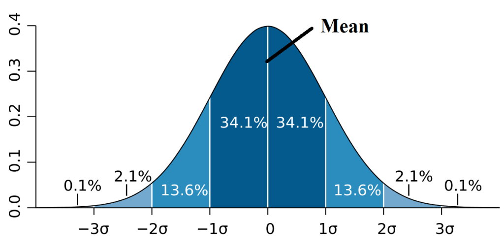
So we flip a coin, the mean value is the most likely outcome for our data, so since a fair coin is 50/50 we would expect to see a 0.5 for the mean value in a perfect world if we flipped a coin 100 times we would get 50 heads and 50 tails. The x-axis has little odd looking o’s which are called sigma and 1 sigma is 1 standard deviation away, the standard deviation is basically a measure of variability in your dataset, so if you were measuring something with high variability you would have a large sigma, low variability would give you a low sigma and 2 sigma away is just sigma * 2, 3 sigma is sigma * 3 and so on.

An aside, but here’s a someone simple explanation for standard deviation. Let’s say we we wanted to figure out the time it took 50 people to run a mile and we knew that it would be a gaussian distribution (we’ll explain how to figure that out in future posts). If they are all runners it wouldn’t be far fetched to say the mean would be 4 minutes, so the average runner did a 4 minute mile. One standard deviation away is done using a bit of math, but you take the mean, subtract the measured value, square the whole thing so it’s now positive, so let’s say you were one of the runners and did it in 4.5 minutes, you would have a value of -0.5 minutes or 0.25 if we square it. We would do this for all the runners and total the values so 50 runners and let’s say the squared sum of all of them is 1.25 (just picking a number). We then divide that by 50-1 (n-1 because we used some of the data to find the mean so our mean is 1 of those data points). 1.25/(50-1) is roughly 0.026 and we take the square root (since we squared everything to make it positive!) and get about 0.16 minutes or ~9.6 seconds. So 68.2% of our runners ran the mile in 4 minutes plus or minus 9.6 seconds!

So what does this have to do with effect size? It turn out that we don’t know what our curve (the normal distribution above) looks like, we don’t have the actual values for mean and standard deviation and we most often will never have the ACTUAL values because we’re looking at a sample and not a population. Using our runner example we sampled 50 runners, but the population is far larger and would include all runners. Since we can’t test every runner alive we take a sample and run our test using that data.

Now let’s go back to our coin example since effect size will be easier to understand using the simple example. Because it’s a fair coin and you have a 50/50 chance of getting heads or tails we can actually find the TRUE mean and standard deviation for our dataset and we’ll look at how to do that in upcoming posts. In fact, you already intuitively know the mean is 0.5*the number of flips, so again easy example.

Now let’s say I give you a coin and we need to find out if it’s fair. But being an evil genius that I am I’ve engineered the coin to give you exactly 1 more heads on average per 20 flips than you would expect to have. In other words, it’s not a fair coin, but 1 extra every 20 flips isn’t heads every time. If you knew this in advance, that is effect size. If I engineered the coin in such a way that every 20 flips you got 19 heads we would say the effect size is large so the mean of the data you would collect from this coin would be shifted to one side or the other.

Let’s say (using the image above) that heads pushed you towards the positive tail (side) and tails pushed you towards the negative tail (side) we would determine the mean and standard deviation of our evil coin to the unbiased population or what we would expect the mean and standard deviation to be if our coin was fair. If we flipped a coin 100 times we would expect a mean close to 50 heads and 50 tails if our evil coin gave us 19 heads for every 20 flips on average we would see that our mean was ~ 95 heads and ~5 tails. Our effect size is huge because the coin is incredibly bias, so we can see right away that we are far from the true mean (50/50).

Now let’s say we did the same thing but with the sneaky coin that gave you 11 heads and 9 tails for every 20 flips on average. If we flipped the coin 100 times you would end up with ~ 55 heads and ~45 tails. Even though I told you that for sure our coin is bias, the effect size is low. So low in fact that (I didn’t calculate this so I’m not certain) if we used a 95% confidence interval to determine if the coin was fair or not, we may walk away thinking it’s a fair coin. Again, without doing any math and making the numbers up, we know a coin should be ~ 50/50 and let’s say 1 standard deviation for 100 flips was 3 so we could get 53/47 or 47/53 heads to tails with 1 standard deviation away. Our 95% confidence interval is 2 standard deviations away so we would expect a fair coin to be 56/44 or 44/56 heads to tails and our result falls in that confidence interval.

To see a small effect size we need more data. We would need to flip it 1000 or 10,000 times before we had enough data for the bias to show itself because our standard deviation values would change and our coin would show increasingly that it was bias (about +1 head for every 20 flips, so the more flips the more the data drifts to more heads). This is why in physics they use such a high confidence interval (the 99.997% confidence interval) to be sure, they need a ton of data because the effect size is incredibly tiny. Imagine if our sneaky coin was bias, but only 1 extra head every 100 flips or 1000 flips on average, it would take an incredible amount of data to show that it was bias (because the bias accumulates for every 100 or 1000 flips we get 1 extra heads).

Simply put, effect size is a measure of how far the normal distribution of our collected drifts away (the header image demonstrates this) from the “true” mean and standard deviation. The more overlap there is, the harder it is to tell the two apart. If we had a very bias coin and got 99 heads our mean would be shifted so far right there would be little overlap, if we had a coin that gave us 55 heads our mean would only be shifted slightly from the “true” mean of 50 heads.

Now this isn’t exactly a “real world” example, I can’t actually bias a coin like that, but it gives you an idea about why effect size is so important. Keep in mind, because we can’t tell what our effect size is without collecting data, we normally have a control dataset and what’s called a “treatment” or “intervention” dataset.The treatment or intervention dataset is just the new thing we’re testing, the reason for the experiment basically. In human experiments, like what I do, we usually try to use a control condition on the same person to account for individual variability. Then we can build the curve above using the control data and compare it to our treatment data. This is why we do pilot experiments, to figure out effect sizes prior to doing a full experiment because we can determine approximate effect size and how many participants (data) we need to conclude if something is working or if it’s just random luck, which does happen!

In my line of study using electrophysiology (how the body responds to electrical stimulation), our effect sizes are often large enough that we can see differences with as little as 5 to 10 subjects. Sometimes even with humans you need far more though, for a good fMRI study, they typically (from my understanding) use 50 or more subjects because the effect size is much smaller and you need high confidence in your findings.

Tomorrow we’ll introduce the central limit theorem and really discuss the idea of the normal distribution (or gaussian depending on your preference). Then we may finally (FINALLY!) be able to look at some of the math and do some testing with our coin to tell if I’ve given you a fair coin, or my super sneaky bias coin. *Insert evil laugh here*