The central limit theorem in statistics

Today we’re gonna push it to the limit! The central limit theorem that is. It’s a cornerstone in statistics and the short and dry version is that it lets us turn any distribution we have into a normal distribution. If it wasn’t for the central limit theorem statistics would hurt far worse than it does now (speaking as someone taking a stats class now). For the longer version we need to discuss why a normal distribution is needed, why we prefer to work with them!

It was about four weeks into this class that I asked myself what I was doing here. I hate math. Okay, I don’t hate it, I just prefer to understand more about it than just the equations. I didn’t become an engineer just to plug numbers into an equation, I wanted to know WHY! If you’re like me, you just get things better when you know the why behind something, that’s what this series is, a behind the scenes look at the why. A little bit about me, third year PhD candidate in neuroengineering, I have a BS and MS in mechanical engineering and I do math a lot! the “in statistics” posts are for anyone looking for an intro into the subject, if your more advanced you may find it useful too.

What is the central limit theorem? It would be helpful to define it in a way that would make sense to the average person. The central limit theorem says that if we have a population and take a large enough samples from it (typically n > 30) with replacement (defined below) no matter the distribution of the population, the sample we took will be normally distributed! If the distribution is already normal, then it will hold for samples n < 30 too, but frankly we don’t always know the population distribution prior to testing so better to be safe!

We just used a lot of terms that may not be properly defined so let’s go over that first. With replacement is just like it sounds, let’s say you have a bag full of marbles of different colors. If you wanted to sample that population of marbles you remove as many as you would like, if you’re sampling with replacement, you are simply putting the marble back before you shake it up and draw a new one. A population is the whole group of the thing you’re interested in, if I wanted to find the average weight of a wild rhino for example, the population would be all wild rhino in the world and my sample would be the rhino I’ve somehow managed to weigh.

Now, chances are rhino weights will be normally distributed already, but let’s say they weren’t, let’s say they were a poisson distribution (they definitely aren’t, but just go with it). The sample I took from the population will be normally distributed (assuming I took a random sample and didn’t weigh the same 3 rhinos 10 or more times). That’s the sneaky thing about statistics, you can bias your result by taking a sample from a bias population. Imagine I polled people’s preference between Captain America and Ironman, but I did it at a Ironman fan convention. I would most likely end up with a lot of Ironman fans and would conclude that more people liked Ironman than Captain America. You need to be careful about how you take your sample in other words.

Very quickly what do other distributions look like? Well there are a lot and they all describe different things, most biological processes are normal and I’m thankful for that! Others, like waiting for a train for example (assuming arrivals are random) we use a exponential distribution. Flipping a coin is a binomial distribution (because there are only two outcomes), so you have a lot of different distributions you’re working with and below is a figure of what the probabilities look like for them.

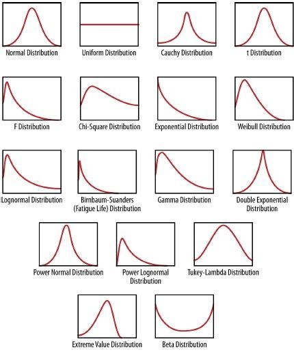
Keep in mind the y axis is your probability so the bigger the value, the higher the chance you’ll fall in that area under the curve, your x-axis depends on the problem. If we’re talking weight of a rino, then it’s your prefered unit for weight, running times is you prefered unit for time, etc. We have a lot of distributions, but the central limit theorem says that if we take a sample, we’ll get a normal distribution and we like the normal because it’s easy to work with.

Unlike other distributions, with just two different variables we can describe the entire distribution. All we need to know is the mean and standard deviation and we know exactly what the distribution looks like (it will always be bell shaped, but the standard deviation dictates how wide that bell looks). A lot of regular statistical tests we run require us to have a normal distribution, so if we want to test for example if a coin is fair we need a normal distribution, (or the approximation anyway), same thing with anything we’re doing.

Note, there are statistical tests that do not have this requirement! Those are called non-parametric tests and we will (probably) touch on them some time in the future, but for now we normally use parametric testing, if you do any sort of stats it will probably be using parametric tests, and that is why the central limit theorem is so useful, it all becomes normal. This isn’t so useful for testing against a known population, but like I said before we don’t usually know the true population statistics. What we usually do is take a sample from one group and a sample from a second group, now we have two normally distributed samples and can compare between the two even though the population they came from isn’t normal, pretty cool, right?

So now that we understand why the central limit theorem is so… central, to statistics we can move on to doing some testing! Tomorrow we’ll test a coin and determine if it’s statistically fair or not. Maybe I gave you a coin that gives you all heads, or maybe it’s the sneaky coin that gives you 1 more head than expected every 20 flips, you’ll have to wait and see! In the meantime, here’s a little visual showing how random processes tend to be normally distribution, this is of course a binomial distribution which tends to be fairly close to the normal anyway, but it’s a good demo of the theory in action. I should mention it’s binomial because the balls can pick either left or right (heads or tails) at each peg they hit and each time is independent of the previous peg it came in contact with. So this is a good example of why flipping a coin a lot is approximately a normal distribution!