The t-test in statistics

Welcome fellow mad scientist enthusiasts, the last time we talked statistics, we found ourselves in an interesting situation and we need to figure out if the mind control device that was developed is actually working. We introduced the idea of a two population problem and today we’re going to use something called a t-test to determine if our mad scientist succeeded.

A quick introduction for those of you wondering what’s going on. I’m a third year PhD candidate in neuroengineering, I have a BS and MS in mechanical engineering, and for the past two years I’ve been blogging about my PhD journey every day. Lately I’ve been talking about statistics because it’s the last required class I have for my PhD and because it’s good for me to make some notes of all this! This post is a continuation from the other days talk and basically builds on all the “in statistics” posts I’ve made (in the math category for anyone who is trying to catch up). I’m still trying to learn all the nuances of stats, but this is a good way to make some notes and hopefully (assuming it’s all correct!) help others learn as well.

Let’s recap a bit, our mad scientist got funding to build a mind control device (if only it was that easy…). They want to test the device on people and it looks like it may be working, but not 100% of the time so we need to figure out if it’s really doing anything. Even if it doesn’t work 100% of the time, this technology would be beneficial to the mad scientists plans of world domination, so how do we test the device?

We came up with several different study designs to test this and covered some of the problems with different paradigms. For simplicity’s sake, we decided to test 30 people and split them into two groups, the first group started the experiment as the control and the second part of the experiment we tested the effects of the mind control device. The second group got the mind control device first, then no control for the second experiment. Importantly (but not touched on) our subjects had no idea which groups they were in, we call this blinding and we didn’t blind our researchers, but we could’ve (and often do).

Because we’re doing human testing and preferences can be affected by dominant hand (maybe) or a lot of other things, we decided that even though we have two choices for selection (success/fail) like we did with the coin flip, but we think (we don’t know) this isn’t the same as a fair coin test because of that (possible) left/right preference. So we need to estimate the population statistics of left/right preference before we can determine if our mind control device is really working (to determine effect size).

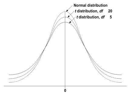
Before we dive into the math, what the heck is a t-test? The t-test (student’s t-test, named after the guy who developed it) uses the t-distribution, which (of course) looks almost exactly like the normal distribution, but has larger tails (the ends) so there’s slightly more variability at the ends of the curve, below shows an example of the t-distribution. The more subjects you have, the more the t-distribution looks like the normal distribution and it’s typically a minimum of ~ 30 subjects to approximate the normal.

The t-test gives you something called a t-score which is just the ratio between the difference between two groups and the difference within the groups. The larger the t score, the more difference there is between groups. The smaller the t score, the more similarity there is between groups. To make matters slightly more confusing, you can also get a p-value from the t-test which is just another way of telling how different the groups are. Unlike the last example though, the t-test can be used with two samples (the two groups we’re testing). It’s a subtle difference, but in this case we don’t know the population of either of the groups, we only have our samples so we can’t use the same test.

Now that we have an idea of what the t-test does, let’s talk about how it does it. The (in this case paired, we also have a pooled version) t-test looks at the differences between the groups, in our case each group had 30 subjects (since we tested the mind control device on both groups, just at different times). All we do is number our subjects 1-30 and subtract the first session from the second session! Seriously, that’s half the battle. so if we say success is 1 (grabbing the object we want them to grab) and failure is 0 (grabbing the alternative object) and each session we tested our subjects a total of 10 times (a repeated measures test, which we’ll get into…eventually), we would have something that looks (shortened) like this:

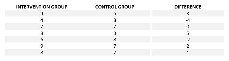
Meaning for row 1 the subject during the intervention portion (the mind control device) selected the object we wanted 9 out of 10 times and in the control session only took the object we wanted 6 out of 10 times. Literally in this case we’re interested in the differences (last column) and you’ll see why below as we introduce the t-test calculation. The D in the equation is the difference (from difference column). Notice how I seperated my data into control session and intervention session, since we tested half in one session, half in the other and then flipped the groups, we need to organize our control and intervention (mind control) tests to determine the differences. N is the number of subjects (or in this case data points) in each group so since we had 15*2 data points, we have an N = 30, even though it’s repeated measures (again we’ll cover what that means some other post, just know it exists).

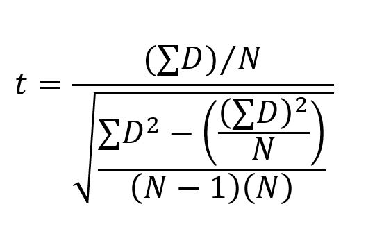
So we sum (the backwards almost E looking thing) the differences, divide by the number of data points we have (N). For the bottom half of the fraction we are dividing that by, the absolute value of the differences, which is the reason for the square of the differences (D) then subtract the average difference (which is what we’re doing by dividing by N) the whole thing gets divided by (N-1)(N), which the denominator (the bottom of the fraction) is just the variance of the difference. Overall this is just the mean of the difference divided by the variance of the difference.

The output t is something called the t-statistic. That number then gets mapped to a p-value, there’s a formula for it I’m sure, but we either use software these days or if you want to go old school we have tables! Fun fact, log calculations (log10(x) for example) are easily done on calculators, but there used to be whole books full of log values. Anyway I digress, back to our problem at hand… our p-value (like before) is our chance that we made an error so if we want a 95% confidence interval, we set our p value to be less than 0.05.

On to some numbers! We could calculate all this by hand if I gave all the numbers we needed or I could give the sum of the differences (D) and since we know N = 30 we could plug and go, but let’s skip that and just look at the t statistic part. Let’s say we run the numbers and get a value t = 1.41.

First we need to explicitly state this is a one tailed test, I haven’t covered that, but I will in detail eventually. The short version is one tail means we only care that our value is greater than the control group (or lower, but not both higher or lower), since we assume our mind control device isn’t causing the opposite effect (making people chose the object we don’t want them to chose) we look at the 1 tailed test. There are tables for both and it’s easy to go from one to the other (again we’ll cover it probably tomorrow).

Since we had a N = 30 our degrees of freedom (DOF) is 29 to use the table find your DOF and then you look for where your t-value falls. This table is a condensed version, but you can calculate your exact p-value using software like R, MATLAB, or a number of other statistical software out there. This is just an easier way to show how to use the table. The table below highlights how we find out if our value is “significant” or not. Notice I highlighted the DOF = 29 row, follow it over until you find the values where your value falls and you have your “rough” significance.

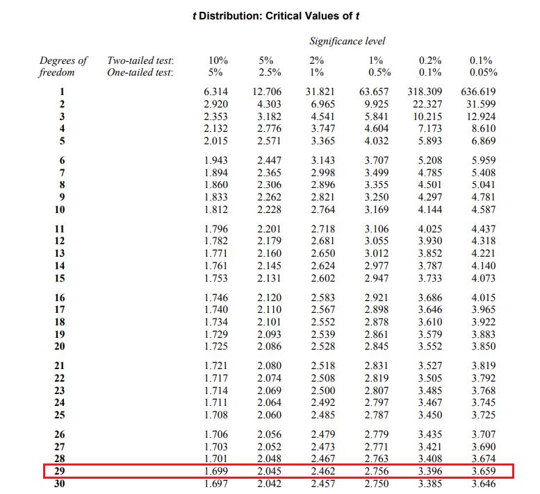
Since our t-value is 1.41, the first value is at the (one-tailed) p = 0.05 level, which is what we’re trying to hit. We needed a t value greater than 1.699 to have significance, so we say that we CANNOT reject the null hypothesis (remember we never accept it, but that’s just the convention, we use, it isn’t wrong exactly). Because there is no statistical significance between the group we conclude that our mind control device wasn’t working after all! At least not with the statistical power we had from the experiment meaning the effect size is either small, or it doesn’t work. Because our mad scientist wants a device that has a high effect size, we won’t be testing this device again. Unfortunately, it’s back to the drawing board for our mad scientist.

A few caveats to our t-test! To the t-test we need the variances between groups to be equal (or at least very close), we need independent and identically distributed data (which assumes we took our samples at random), and lastly we need to either check or know that our data are normally distributed. There are tests to check for normalcy and for variance differences, we’ll have to cover those some other time though!