Confidence intervals in statistics

Well since our mad scientist from yesterday’s post is on a short break, today we’re going to fill in some of the gaps that post brought into view. First up is the confidence interval. There are some subtle points here, so this should help clarify a few things that may not have been clear yesterday. We’re going to do a somewhat deep dive into what the heck we’re doing when we talk confidence interval and why the standard deviation of our data is important in determining the values.

Statistically speaking no one understands statistics. I mean math can be hard and if you’re like me if anything is going to stick in your brain you need to know the why. If you’re just joining in, this “in statistics” series should help clear up a lot of the why, as in why are things that way and not some other way, why does this work, why am I such a failure! Okay, that last one is a personal why, not a statistics why (kidding… semi-kidding… fine, very serious). Who am I? Well I’m a third year PhD candidate in neuroengineering and I have a BS and MS in mechanical engineering. I blog daily about my journey (for the past two years anyway) and since this is my last required course for my degree, I wanted to make some useful notes for myself and anyone else who may be struggling with the same statistical confusion.

The idea of the confidence interval is very simple. It’s literally how confident you are that your result isn’t an error. This can be done in shorthand one of two ways, you can say you have a 95%, 99%, 99.9%, etc confidence, or you can say your p-value is less than 0.05, 0.01, 0.001, etc. and they are two sides to the same coin. In the first example you’re saying you’re 95…99.9% confident that you did not make a type 1 error. We can (and do) also say your p-value is less than 0.05,..,0.001 which translates into the likelihood you made a type 1 error is 5%,… 0.01%. Remember you need to convert your p-value to percentage if you’re doing that (just multiply by 100), but the shorthand p < 0.05 works just as well for those in the statistics field or who have an understanding of stats.

The real question is where the heck does that come from? In statistics a lot of things we do revolve around the normal distribution, the t-test for example requires your data to be normally distributed or the math doesn’t work. The central limit theorem helps make everything normally distributed so that helps (in some cases!!!!!!!! We will touch on that eventually as well). As a refresher, let’s look at a normal distribution curve.

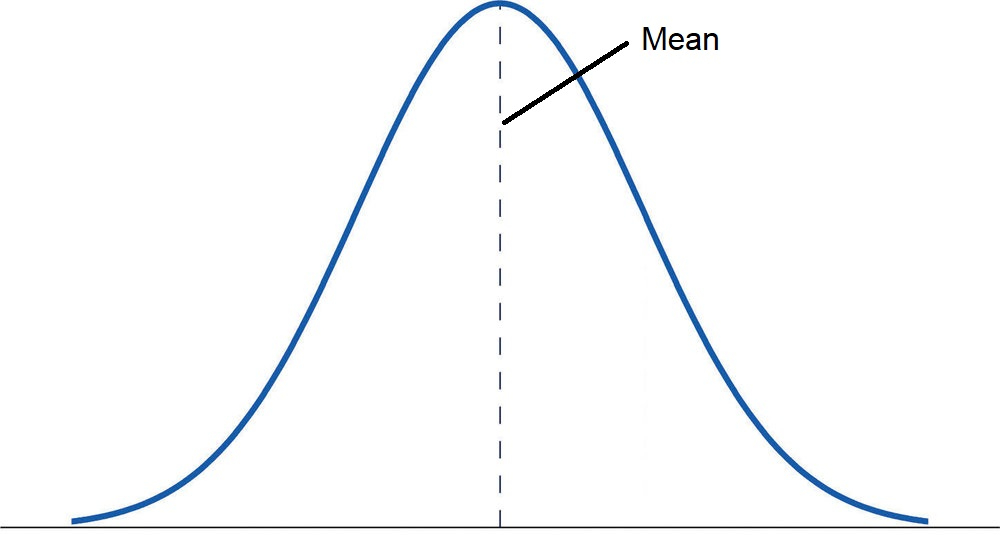
There’s a lot going on in this seemingly simple image so let’s highlight what those things are, first you have two tails, those are where the curve stops, notice how I didn’t say end! The drawing stops, but the curve gets closer and closer to the zero (the solid x-axis line) as you approach infinity (right tail) or negative infinity (left tail). The dotted line is the mean, which I’ve labeled here for you. The area under the curve is probability, so the probability you will hit the mean is the highest point because (drum roll) it’s the mean, or the average of the numbers so this bell shape will be centered around the mean. As we move away from the mean the less likely you are to have the event occur. If I flipped a coin 10 times and got 5 heads, we would be directly on the mean, if I flipped a coin 100 times and got 100 heads, then I would be far off to one side of the tails depending on if we called heads success or failure (like really far off because the likelihood of that happening is incredibly tiny, but as with all things in statistics never zero!).

That’s why we need to calculate the standard deviation of our data, that determines how wide the bell shape is. If we had zero standard deviation we would just have a line at zero until we hit the mean, then it would shoot to 1 and drop back to zero for the rest of the values. Conversely if we had a huge standard deviation our shape would look incredibly wide and the peak (at the mean) would decrease. Below is a good example of what that looks like as the standard deviation increases.

This is a good image because as you see, the y-axis is labeled density, that’s probability density and if we look at the red curve (the highest curve) the probability you’ll get a mean value (100) is about (eyeballing it) ~ 0.175 or 17.5%, but the chance that you’ll get a value of 87.5 is very close to zero (again it never actually hits zero until you approach negative infinity or positive infinity, it just gets very, very, close.

Our actual values that give us a 95,..99.9% confidence interval is then effected by our standard deviation. A high variance will return a wider spread of values to give you your confidence interval while a low variance will give you a small spread. For example say our 95% confidence interval for the red curve is two standard deviations from the mean, the variance is 9 and you may recall that variance is just standard deviation squared, so we take the square root and you’ll see pretty easily that one standard deviation is + or – 3, so our 95% confidence interval is 2*3 or 6. We then subtract and add that to the mean to give us the confidence interval in both directions of 100-6 = 94 and 100+6 = 106. Now we know that we have a 95% chance of getting a value between 94 and 106, often written as [94 106].

However, if we do the same thing for the variance of 100, we take the square root and find our standard deviation to be 10, so our 95% confidence interval is 2*10 = 20, then add and subtract that from the mean value, so 100 – 20 = 80 and 100 + 20 = 120. Which means our 95% confidence interval is between 80 and 120 or [80 120].

So we can see just by this simple example that if we have 100 data points and find the mean and variance we can determine pretty easily where 95% of the values will fall so if we take a different set of data from a different group (but same population) we should see 95% of the values fall within our confidence interval. If they don’t then we found something different between our sample and the population (IE our fair coin or mind control experiments).

Here’s the subtle part though, we have 5% chance of making an error in either direction. That means we could have data that fall (using the last example with the larger variance) above 120 OR below 80. So the total error in both tails is 5% meaning that the error in only one direction, let’s say above 120 is 2.5%.

A short example, say that we use the data from the figure above and the wider variance (variance = 100). Say that data is test scores and we want to see if a new method gives us higher scores than the method used above. Well we don’t care about the lower tail, so we can perform a one-tailed test and look at the higher (or lower depending on your application, it can be either direction). Well we would no longer use the same confidence interval we just found because as I just said only 2.5% of the error is contained in the higher tail, so we adjust our confidence interval to negative infinity to whatever value the 5% error would be (I’m not calculating it, but feel free to try it yourself!). This would give us a lower value than the 95% for a 2-tailed test (the values we calculated above), so without finding the value we already know our confidence interval would be negative infinity to some number less than 120. To find the actual value you need to calculate it though because it isn’t as simple as basic math, there’s a formula that goes into the curve, but there are tables to help!

The table will tell you if it is a one tailed or two tailed table and now you know what that means. Sometimes a one tailed table will give you only one direction (the negative direction). That’s okay though because the probability of ending on the other side of that value is just 1- the value. Normally this is going to be a z-score or a t-score depending on what calculation you’re using (z-score when you know the population standard deviation like our coin toss example and t-score when you don’t know the standard deviation of our population and have to use a sample to estimate it, like the mind control example).

Hopefully this post gave you some confidence in confidence intervals! Yes, that was a bad pun, please don’t write angry letters, I’m already PUNishing myself… see can’t help it, bad puns left and right. I’m not sure quite yet what the plan is for tomorrow, but hey that’s the fun of it sometimes. As always, feel free to add any of your own thoughts or tricks that have helped you! I would love to get others insight.