The p-value in statistics

We’ve been dancing around the p-value for some time and gave it a good definition early on. The p-value is simply the probability that you’ve made a type one error, the lower the p-value the less chance you have of making a type one error, but you increase your probability that you’ll make a type two error (errors in statistics for more). However, just like with the mean, there’s more than meets the eye when it comes to the p-value so let’s go!

We use statistics all the time, we take guesses and try to figure out probabilities pretty much on a daily basis. Like the probability you’ll get your work done (0% since it’s a pandemic life), the probability this zoom meeting will end soon (again 0% chance because pandemic), or the probability that I’m making a horrible joke (100% because it’s me, I’m a horrible joke). The point is that statistics is useful, from voting outcomes to vaccines, we need statistics to tell us if something is working, to predict food consumption, weather, tides, traffic, public transportation needs, and just about everything else that we deal with. Since statistics is everywhere, it’s easy to get sucked into pseudoscience claims using statistics if you don’t understand how the methods work. Thankfully that’s what we’re doing with this series, trying to understand why statistics works and is the way it is.

First a quick review, yesterday we talked about the z-score, which we said was just a measure of how far our value was from the mean in standard deviations. We also said that our standard deviation isn’t a fixed value, but a value that depends on the variability of our data (how spread out our measurements are). We also said that the concept was important because we could say how likely an observed value was caused by randomness (likelihood of a type one error) or if it was actually significant by how many standard deviations away from the mean it was located.

For example, when dealing with normally distributed data, we know that the amount of data located one standard deviation away from the mean (either plus or minus) is ~68.3%, if we go out to two standard deviations away from the mean we find ~95.5% of our data, etc. Remember, this never changes, one standard deviation away from the mean will always contain ~68.3% probability, it’s the size of one standard deviation that changes, for example one standard deviation from the mean could be 5 or it could be 50, but in either case it’s still just one standard deviation away. This tells us something very important, if our observed value is more than two standard deviations away from the mean then we can say that there is at LEAST a 95.5% chance that our observed value is significant and not caused by randomness of the system.

However, just like there are different units to measure with, there are also different ways we can determine significance. The z-score is (in my opinion) very intuitive, it makes sense, it’s easily calculated, and we don’t have to rely on tables to tell us if our value is significant, we can just see it based on how far away from the mean we really are. The z-score has, let’s call it a sibling, and sibling that is p-value. P-value is sort of like z-score in they both tell us how significant our observed value is, however instead of counting the standard deviations away p-value uses percentages.

This may make you think that p-value stands for percent value, this isn’t the case, although it may help to remember it that way. P-value actually stands for probability value. We covered what the standard is for selecting a p-value, that was p-value = 0.05. We also talked about cases where that isn’t always the case, like particle physics, or where p-value doesn’t hold and needs to be adjusted using the bonferroni correction, which we should probably define sooner rather than later (maybe even tomorrow). So let’s look at the z-score formula once again.

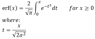
Using our z-score from before, we can calculate the p-value and there are several different tables or even functions in software like MATLAB, Rstudio, excel (yes, that excel, the windows software) . There is an actual formula for you to calculate it directly, however really what you are doing is calculating the z-score then either using the table or if you’re pretending you’re stuck on a desert island and are that bored, there’s a formula for it, but it involves something called the error function and for completeness, why not! Let’s go wild like it’s a Friday night and throw out some equations (this is why I never got invited to parties):

Now the formula above would spit out the probability of getting a value up to a certain x (the x value you have), so a one tailed text because we’re looking all the way back at – infinity to a certain value, replace the – infinity with a lower bound and you have a two tailed test, easy… okay not really. We’ll have to define the one and two tailed test some other time so we can cover it in detail, but basically a two tailed test is looking for the probability the value you measured falls between a range like P( 10 < x < 20) or the probability that x could be between 10 and 20 given your distribution (vs. the one tailed example I just gave from – infinity to a value).

The erf, that’s the pain in the ass error function (okay it’s not THAT bad) and that guy looks like this:

But really, all we need is our t-value (not the t from the error function mind you), f-value, or our z-score, and we can easily find the p-value. Hence why we said that the z-score and p-value are related, but if you want to get technical it’s all related.

One last reminder before we wrap up, a p-value of p = 0.05 really means that there is a 5% chance that your observed value was caused by randomness. In other words, when used properly (heavy emphasis on properly) you have a 5% chance of making a type 1 error. Which is why p-values are more commonly used when talking about your results because p = 0.05 is easier to understand in that sense than trying to explain that your data point is 3 standard deviations away, it basically means the same thing, but think of it as phrasing your result in a different way.

Well that’s all we have time for today. Next up we may be talking about the bonferroni correction or maybe we can cover the difference between a one and two tailed test since we are back on the “in statistics” kick, who knows! In any case, it feels like we did a pretty good job covering what a p-value is and how it works, hopefully this was useful.