The Tukey test in statistics

No, not turkey, Tukey, although they are pronounced very similar (depending on who you ask I guess? I’ve seen people pronounce it “two-key”). Any way, today we’re saving our job and the wrath that comes with failure. The mad scientist boss of ours tasked us with testing mind control devices and determining statistically which one (if any) worked. After the last failure, we now had four new devices to test, so we couldn’t use the same method as before. However, an assistant’s work is never done, we didn’t finish the job! That’s what we’re going to do today.

I absolutely hate the way the sciences are taught, in the general sense. We often learn the formula, the ways to apply it, the limitations, and are expected to go into the world wielding that knowledge without ever questioning where it came from. Why is it one formula and not another? Why does it work? Why are there limitations and assumptions if it’s math? Maybe it’s the rush to cram as much information into our heads while in school as possible, but I for one never could grasp how to use the tools without understanding why the tools even worked. I mean that’s why I’m an engineer, I take things apart and put them back together in different (and hopefully) better ways. So that’s what this is, my attempt to explain the why, for me and for anyone who can’t seem to use the math without knowing what the heck it’s doing.

A quick recap to how we got here before we dive into today’s topic. Each post of my “in statistics” series builds off of the previous posts, so you may want to start at the beginning (here). Because we’re poor college students, we decided to take work in our local mad scientist’s lab to earn some extra cash. They tasked us with testing a mind control device using statistics, so we applied a t-test and found it didn’t work! Undeterred, the mad scientist came back to us with not one new device, but four! We needed to test them all to figure out which (if any) were working. We couldn’t use a paired t-test, because the error blows up and suddenly we have no confidence in our findings, so we used a one-way ANOVA. The catch? The ANOVA only told us there was a significant difference, not which device was significant!

That’s why, in order to save our jobs, we’re going to solve this using the Tukey test or the full name the Tukey’s Honest Significant Difference test (sometimes abbreviated Tukey HSD, or just HSD). Before we blindly apply the test to appease our mad boss, we first should dive into the workings of the Tukey test and explain what it does.

The Tukey test tests all pairwise comparisons of our groups of data to determine WHERE the significance is coming from (there may be multiple significant pairs). Now yesterday we said we couldn’t do that with the t-test because our alpha, or the chance that we made a type 2 error shoots up dramatically as we start adding more and more comparisons. This is why we use the Tukey and not t-test, the difference? Well here’s the t-test, let’s compare that formula to the formula for Tukey.

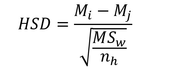
See, different. Now let’s talk about those differences to get to the why this works. The t-test looks at the sum of the differences between the two samples we’re comparing. Here we’re just taking the mean of sample i minus the mean of sample j. Those are just indices so i could be the control and j could be device 1, or any combination you can make from the five choices we have (device 1-4 and the control sample). When we do this by hand (why would you!?) you need to remember have M_i be the larger of the two means for this to work. Now here we’re dividing by the MS_w or mean square within (which, hint this is why there’s a square root involved!). The formula for mean square within is:

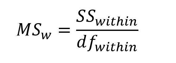
Which we saw in the f-statistic and again in the ANOVA, but we didn’t get into too much detail. Don’t worry about the within subscript, that just means we’re looking at the stuff within the group not between the groups, think total (within) not difference (between). The SS_within is the sum of squares within and is the variance (standard deviation squared) of each group (see total, not difference) multiplied by the degrees of freedom for each individual group (n-1). Because we’re using standard deviation here, we take the square root above to determine our actual value. The df_within is the degrees of freedom within our samples, so sum of our data points – number of groups, in this case that would be n-2 since we’re comparing two groups. Going back to our HSD, we still have the MS_w divided by that n_h. So we should define n_h which is just the number of datapoints in our group, often called treatment.

If we squint hard enough, this almost looks like the difference in means divided by a fraction of the standard total standard deviation and the number of datapoints in our treatment (two samples). Where the t-test is basically creating a third distribution (a difference distribution) to see where on that distribution our mean falls to determine if we have something significant or not. In this case we’re doing something similar, but still very different in that we’re using the difference in just the means of our two samples to determine how different they are from each other.

From a statistical standpoint (and we may go in depth in this because it’s important) the mean is what we would expect to be the “true” value of our data. In short, with the Tukey test we’re comparing means and not pairs of values (like the t-test does), which Tukey (the guy the test is named after) felt was a more “honest” comparison, hence the full name of the test. We already saw a good example of why it’s not really “honest” to use multiple t-tests, the alpha explodes!

The HSD gives us something called a q ratio (notice we’re dividing so we’re creating a ratio just like with the f-test and ANOVA). Which means we can go to our handy q-table to find the “critical value” that will tell us if the differences between treatments is significant. To read the table we need to know our “k” and degrees of freedom. We already talked about degrees of freedom (total number of datapoints – number of groups), but what is k? In this case, k is the number of groups we have, so for our example we had 1 control group and 4 mind control devices giving us a total k = 5. Since I’m going to be doing this example using Rstudio, I won’t be highlighting the columns or rows, but I will go through how to find the value and give you a quick example below.

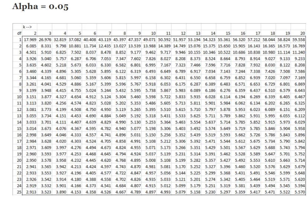
As mentioned previously, the columns are the k value and the rows are your degrees of freedom (df) so if we had a total of 30 participants our df = 30 -5 = 25 and our k = 5 so our critical value is 4.153 (the k = 5 column and follow it down to the df = 25 row). That was just an example though, I never explicitly stated how many participants we had in this study, sort of on purpose.

So now we know how it works, why it works, and why we use it instead of just t-testing our way through the whole mess. Let’s use the data previously shown to figure out where our significance came from. I’ll put the bar graph of our dataset here to remind you, but you can also review the ANOVA example to get an idea of what’s going on.

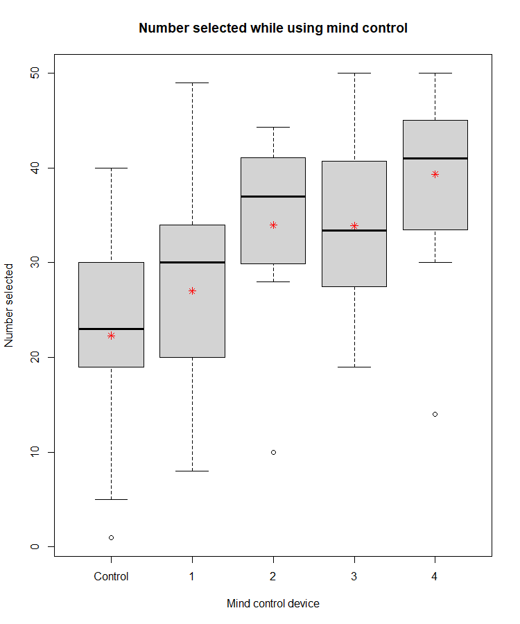
So yesterday I just eyeballed the plot and said it looked like mind control device 2 and 4 seemed to be working when compared to the control. Our mad boss wouldn’t be happy with that though, mad scientists are sticklers for statistics, so we can use the tukey test to find WHERE our significance is coming from. As a reminder, the mean is the red asterisks (*), the median is the dark black line, and the minimum and maximum values are the ends of the dashes, the single points are considered outliers (which in the software default means they fall > 2 standard deviations away from the mean value). Yesterday I didn’t give any of the Rstudio commands since I hate Rstudio and probably will never use it after this class, but my hatred aside, it may be helpful to those who use it regularly to cover what I’m doing. The R commands for your ANOVA (since I didn’t include them) are:

Which is just loading my mind control data (the first line), setting my “factor” as the group (which I called device, even though technically it has my control group in there too) from my mindcontroldata dataset. As a quick note, your factor is how you broke up your data, or the groups. Now we can do the analysis (analysis) which calls the ANOVA command (aov) and I’m comparing my number selected (mindcontroldata$nselect, which looks inside my data for the column named nselect) to the device used. Summary gives us the output from this, which is what you saw yesterday.

Now that we’ve covered that lets do the same, but for the tukey test.

Since the tukey test is a post hoc test (post hoc means after the data is collected) I called my output posthoc, so that’s where the results will be stored. The R command for the tukey test is TukeyHSD, the first input is from my ANOVA (analysis), the second is what I’m comparing (the mind control devices, or “mindcontrolfactor” as I call it here), and lastly I set my confidence interval. Then I call the variable posthoc and it spits out my results which are:

We had 5 groups so 10 tests total and the last column is where we have our significance, which is given to us in our very familiar and very useful p-value! So we just scroll through those values and see where we have significance. The fourth p-value down (0.0001865) is definitely significant! So if we follow that row back to the first column we see that the two things being tested are group 5 and group 1. Group 1 is our control and group 5 is our fourth mind control device so it looks like we have a winner!

You’ll notice one other value made the cut (p = 0.0096) and that is 5 and 2 or mind control device 5 compared to device 1, but that just means device 4 was significantly better than device 1 which doesn’t do much for us because device 1 and the control were basically the same! Two other values came close to making the “cut” so to speak (p <0.05) we have 3 and 1 (p = 0.0541…) and 4 and 1 (p = 0.0564) which are devices 2 and 3 respectively, compared to the control. However, like good little statisticians we say NO to those and go with the one that gave us a very significant difference when compared to our control!

In the end we learned why the Tukey test is important, how it differs from the t-test, and our boss will be very happy that we have a successful mind control device for world domination! Hopefully with this good news, he won’t try to dissect us again…