We're a little crazy, about science!

Latest

Day 42: Conditional Probability

Conditional probability pdf plot

How does this not exist on the internet?! This is directly from my book, so it looks a little… well loved.

Up to now we’ve been dealing with single variable pdf and the corresponding CDF. We said that these probabilities relied on the fact that our variable of interest was independent. However, what if we knew some property that impacted our probability? Today we are talking conditional probability and that is the question we will be answering. It’s going to be a long, long post so plan accordingly.*

Read the rest of this page »

Day 41: Connecting the Concepts

catinthebag

Maybe we shouldn’t phrase it this way, since there is still quite a few days left of 365DoA, but you made it to the end! No, not THE end, but if you’ve been following along the past few posts we’ve introduced several seemingly disparate concepts and said, “don’t worry they are related,” without telling you how. Well today, like a magician showing you how to pull a rabbit from a hat, let’s connect the dots and explain why we introduced all those concepts!*

Read the rest of this page »

Day 40: The Normal Approximation (Poisson)

Poisson vs Gaussian

Poisson’s return!

You have all been really patient with seeing how we tie these last few posts together and frankly I think that we are on track to do that in the next post. Today however we have one more thing to introduce then we can bring it all together, that would be yet another normal (again we usually refer to this as the gaussian) distribution. If you recall I hinted at this a few days ago in the Poisson pdf post.  Let’s look at what this means and why we would want to use this.*

Read the rest of this page »

Day 39: The Normal Approximation (De Moivre-Laplace)

Binomial_distribution plot

The binomial distribution, don’t worry we’ll get into it.

Well we haven’t covered the binomial distribution, but it should be vaguely familiar if you’ve been keeping up, specifically if you’ve already read about the gaussian pdf. Today we are going to talk about what the binomial distribution is and how it relates to the normal distribution. So let’s get into it and see how it relates to some of the topics we’ve been covering!*

Read the rest of this page »

Day 35: Example of the Gaussian pdf

Normal distribution with marbles

The gaussian (or normal) distribution demonstrated by plinko.

Well what a fun day it is! Today we are going to dive into some examples (or maybe just an example) of the gaussian (also known as the normal) distribution. Last post we looked at the laplace distribution and discovered there aren’t a whole lot of uses for it because it is technically a special case of the exponential distribution. This isn’t the case with the gaussian, there are lots of really interesting things we can model using the distribution that are applicable to everyday life, so let’s get started!*

Read the rest of this page »

Day 34: Example of the Laplace pdf

laplace pdf and CDF

The Laplace pdf (left) and the associated Laplace CDF (right). Remember the CDF is just the area under the curve of the pdf.

Last post, we finally got to use the exponential pdf and discovered the math wasn’t completely useless (okay, hopefully by now you know that). However, in the spirit of finding a use for the equations we are covering, let’s look at how we use the laplace pdf. It’s going to be a blast, so let’s get started!

Read the rest of this page »

Day 33: Example of the Exponential pdf

exponential probabilty density function example post

For those who need a refresher, this is a plot of the exponential pdf we are working with today.

Over the past couple of days, I’ve been talking about several different types of pdf and the associated C.D.F. Hopefully, we have a clear understanding of each of those concepts, for those of you scratching your head, I would recommend you start here at this other post. Otherwise, let’s (finally) look at a real life example using the exponential pdf!*

Read the rest of this page »

Day 30: Confidence Interval

Confidence intervals

Yep, we’re talking confidence!

Day 30 already! Where does the time go? It feels like we just started this whole project and it probably wouldn’t be a good idea to look at the remaining time to completion, so let’s not and just enjoy the nice round 30. We will get back to our p.d.f another day, but today is going to be short. That’s what I usually say before typing out 10 pages worth of information so to avoid that, let’s touch on something important, but something I can do briefly. Today we’re talking about confidence intervals*

Read the rest of this page »

Day 29: Probability density functions, Part 3

gaussian CDF vs pdf

Don’t be scared, we’re going to tackle this guy today!

Well, apparently you guys really appreciated my probability density function posts. It’s good to see people interested in something a little less well-known (at least to me). So for those of you just joining us, you’ll want to start at part 1 here. For those of you who are keeping up with the posts, let’s review and then look at specific functions. Namely let’s start by going back to our gaussian distribution function and talk about what’s going on with that whole mess. It will be fun, so let’s do it!*

Read the rest of this page »

Day 28: Cumulative Distribution Functions

Exponential_distribution_cdf

An example C.D.F. of an exponential distribution

Today we were going to do another deep dive into the p.d.f and C.D.F. relationship. Specifically today we were going to talk about specific p.d.f. functions and why we use them, however… I am not doing so hot today, so instead we are going to back track just a bit and talk about what how a C.D.F. differs from our p.d.f. even though we kind of covered it, it would be nice to be clear and I can do this in a (fairly) short post for the day. So that said, let’s get started and we will pick up our p.d.f. discussion next time (maybe).*

Read the rest of this page »

Day 27: Probability density functions, Part 2

PDF_CDF

Today we are looking at our p.d.f. (yes this image has p.d.f. written as PDF, please don’t be confused!) and our C.D.F.’s let’s do this!

Oh hi didn’t see you there. Today is part 2 of the probability density functions notes (posts?), whatever we are calling these. You can read part 1 here as you should probably be familiar with the (super confusing) notation we use to describe our p.d.f. and our C.D.F. now that we’ve given that lovely disclaimer, let’s look once again at probability density functions!*

Read the rest of this page »

Day 26: Probability density functions, Part 1

statisics jokes

Dashing dreams one comic at a time, via Saturday Morning Breakfast Cereal 

We are well on our way to wrapping up week 4, what a ride it’s been! It’s been a long day for me, so today might be short. However, I really, really, really want to break into probability density functions. This topic is going to be a bit more advanced than some of the things we’ve covered (IE more writing) so it will most definitely be broken up. Let’s look at why and discover the wonderful weirdness of probability density functions!*

Read the rest of this page »

Day 24: The z-score

Statistics cartoon

So if you recall from last post… well I’m not linking to it. It was hellishly personal and frankly I’m still attempting to recover from it. We’re going to take it light this time and we can do a deep dive into something in another post. For that reason, let’s talk about z-score and what exactly it is, I mean we used it in this post and never defined it formally, so let’s do that. Let’s talk z-score!*

Read the rest of this page »

Day 21: Defining Parametric Statistics

normal-distribution

It’s halloween time, we are talking about normally distributed data, so this fits, and I don’t want to hear otherwise!

Well my lovely readers, we’ve made it to the three week mark, 5.7% of the way through! Okay maybe that doesn’t seem like a big deal written like that, but hey it’s progress. So last post we had our independence day, or rather defined what it meant to have independent events vs. dependent events. We also said it was an important assumption in parametric statistics that our events are independent, but then we realized we never defined what parametric statistics even is, oops. So let’s stop dragging our feet and talk parametric statistics!*

Read the rest of this page »

Day 16: Type 1 errors

tiny dog yawning

We did it, we cracked the coin conundrum! We managed the money mystery! We checked the change charade! We … well you get the idea. Last post we (finally) determined if our coin was bias or not. Don’t worry, I won’t spoil it for you if you haven’t read it yet. I actually enjoyed working through a completely made up problem, so if you haven’t read it, you really should. Today we’re going to talk dogs, you’ll see what I mean, so let’s dive in.*

Read the rest of this page »

Day 14: Significance, Part 2

Bar graph showing z score across trials

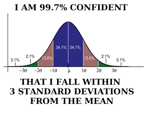
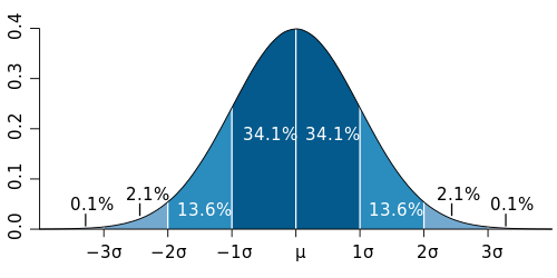
Z-score bar graph that I made just for all of you using some data I had laying around. If you’re new to statistics it may not make sense, but rest assured we will make sense of it all!

Well here we are two weeks into 365DoA, I was excited until I realized that puts us at 3.8356% of the way done. So if you remember from last post we’ve started our significance talk, as in what does it mean to have a value that is significant, what does that mean exactly, and how to do we find out? Today is the day I finally break, we’re going to have to do some math. Despite my best efforts I don’t think we can finish the significance discussion without it and still manage to make sense. With that, let’s just dive in.*

Read the rest of this page »

Day 13: Significance, Part 1

Normally distributed data shown using a histogram plot

Histogram of normally distributed data. It looks very… nomal. No it really is normally distributed, read on to find out what that means and how we can use it.

If you’ve read my last post I hinted that today we would discuss filtering. Instead I think I want to take this a different direction. That isn’t to say we won’t go over filtering, we most definitely will. Today I want to cover something else though, significance. So you’ve recorded your signal, took an ensemble average, and now how do we tell if it actually means something, or if you are looking at an artificial or arbitrary separation in your data (IE two separate conditions lead to no difference in your data). Let’s look at significance.*

Read the rest of this page »

Day 12: Signal, cutting through the noise

example data

45 separate trials of very noisy data with the average of those trials (black). Believe it or not, this is actually very useful and very real data from something I am currently working on.

Noise, it can be troublesome. Whether you are studying and someone is being loud or you are trying to record something, noise is everywhere <stern look at people who talk during movies>. Interestingly enough the concept of noise in a signal recording sense isn’t all too different from dealing with talkative movie goers, so let’s talk noise!*

Read the rest of this page »

Day 11: Why even use the spectrogram?

rotated spectrogram showing all three dimensions

A spectrogram plot rotated so we can see all three dimensions.

So you wanna use a spectrogram… but why? What does a spectrogram do that we can’t do using some other methods for signal processing? As it turns out, there is a lot of reasons you may want to use the spectrogram and today we are going to cover some of those reasons and number four may shock you! (okay not really, what do you think this is a clickbait website?)*

Read the rest of this page »

Day 10: Spectrogram vs. the banana of uncertainty

banana

The banana of uncertainty (okay, it’s not a real banana)

Well ten days in and we’ve just introduced the idea of the spectrogram. While a lot of this information is just the broad strokes, I like to think that we’ve covered enough to give you a good idea about how to use these tools and what they are used for. However, we do need to discuss a limitation to the spectrogram, something called the banana of uncertainty, okay not quite the name, but you’ll see why I keep calling it that.*

Read the rest of this page »

Day 9: Reading a Spectrogram

other example

Definitely not the same spectrogram as yesterday, no really look. Now for the part where I tell you how to read this thing…

Last post we introduced a new tool in our arsenal of signal processing analysis, the spectrogram. Without knowing how to read it, it just looks sort of like a colored mess. Don’t get me wrong, it is an interesting looking colored mess, but a mess nonetheless. Well today we are going to talk about how to interpret the plot and why exactly we would ever use this seeming monstrosity.*

Read the rest of this page »

Day 7: Small waves, or wavelets!

Meyer Mother wavelet

This is the Meyer wave, a representation of a so-called mother wavelet function to use for the wavelet transform. Notice that it is finite!

Waves! We’re officially one week through 365 Days of Academia! Woo! 1 week down, 51(.142…) weeks left! Let’s wrap up this weeks theme (there wasn’t originally a theme, but it kind of ended up that way) by talking about other ways we can get to the frequency domain. Specifically, let’s stop the wave puns and let’s talk wavelets!*

Read the rest of this page »

Day 6: The fast and the Fourier

Fourier_transform_time_and_frequency_domains_(small)

A good example of how the Fourier transform can approximate signals. The red signal is our input signal and the blue shows how the output of the Fourier transform.

Okay, if you’ve been keeping up with these posts, we know about Welch’s method, Thomson’s method, the things that make them different, and the things that make them similar. The thing that both of these transforms rely on is the Fourier transform. What is the Fourier transform? Well, something I probably should have covered first, but whatever this is my blog we do it in whatever order we feel like, so let’s dive in!*

Read the rest of this page »

Day 4: Spectral leakage… embarrassing

Day 4 - Leakage - arrows

Look at that leakage!

Leakage, it’s never a good thing. For today’s post we’re going to cover a very important topic. Spectral leakage, it’s a big reason why spectral density estimation is well, an estimation. The other reason it is an estimation is because the fourier transform is an approximation of the original signal, but the Fourier transform is a whole other post on its own. So let’s talk leakage!*

Read the rest of this page »

Day 3: Power Spectral Density Overview

In our last post we introduced the two main characters in this story of spectrogram. On one end we have Welch’s method (pwelch) on the other end we have the Thomson multitaper method (pmtm). As promised here is a awful basic breakdown of why is more than one way to compute power spectral density (in fact there are several, far more than the two I’m talking about). So, let’s just dig right in!*

Read the rest of this page »

The power of indifference an open letter to the scientific community

indifference

Suddenly your absent-minded thoughts are shattered by a loud noise. Quickly you look around, to the left of you, you see it, and a child has been shot, you see them bleeding heavily. People are standing around with their phones, some calling emergency services, some filming, but most looking confused and scared. No one is actively trying to help; you hear that they are afraid that the person, or persons, who shot the child is still around. What do you do next, do you choose indifference, or do you help?

Read the rest of this page »

The science behind real life zombies

zombies ahead

In the spirit of Halloween we bring you the science fact and fiction behind the undead. Zombies, those brain loving little guys, (and girls) are everywhere. Sure, we are all familiar with the classic  zombie, but did you know that we aren’t the only zombie lovers out there? It turns out that nature has its own special types of zombies, but this isn’t a science fiction movie, this is science fact! Sometimes fact can be scarier than fiction, so let’s dive in.

Read the rest of this page »

A new view of the immune system

t cells

Pathogen epitopes are fragments of bacterial or viral proteins. Attached to the surface structure of cells, they prompt the body’s immune system to mount a response against foreign substances. Researchers have determined that nearly a third of all existing human epitopes consist of two different fragments. Known as ‘spliced epitopes’, these types of epitopes have long been regarded as rare. The fact that they are so highly prevalent might, among other things, explain why the immune system is so highly flexible.

Read the rest of this page »